SUMMARY & DISCUSSIONS

Miscellaneous statistics We have analyzed a sample of 22 limb flares observed by RHESSI, 10 of which have lightcurves of individual LT and FP sources obtained (See Fig. 16 for the distribution of flare locations). Out of this sample, about 6 flares exhibit a classic single loop structure (i.e., with one looptop and two footpoint sources); about 8 have complex morphology; 3 flares appear as a single looptop source. Among the complex flares, we identified one as a multiple-loop events similar to those found by Petrosian et al. (2002); for other complex events further analysis of lightcurves and imaging spectroscopy, as well as multiple-wavelength observation is needed to distinguish individual sources.

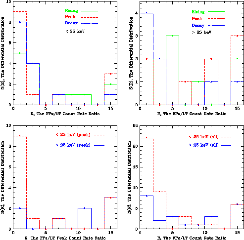
Statistics of the relative fluxes: footpoints v.s. looptops.

• The footpoint to looptop flux ratios reveal that looptop sources are much softer in spectrum than footpoint sources (see the lower right panel in Fig. 17). At lower energies (e.g., $\leq$ 25 keV), the median of FPs/LT flux ratios is very close to 1 ; in contrast, for higher energies (e.g., $\geq$ 25 keV), the median ratio is much greater than unity and its distribution is much flatter. These results are consistent with theoretical calculations (see Liu and Petrosian, poster #16.05).

• At flare peaks, the looptop emission dominates in low energies and footpoints dominate in high energies (Fig 17, lower left panel).

• In the decay phase of a flare (see upper panels of Fig. 17), the looptop source tends to be the major contribution to the total flare emission, especially in low energies (e.g., $\leq$ 25 keV).

Figure 1: The 2092002 flare: lightcurves (left) and hard X-ray images with boxes defined to enclose individual sources (right).

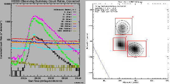Figure 2: Hard X-ray images of the 2092002 flare at different energies. The contour levels are at 10, 40, 70% of the maximum of each panel. The solar limb is marked in yellow. Note the south footpoint is much brighter than the north one, which may be due to possible asymmetric convergence of the flaring loop. That is, the loop may converge much rapidly approaching to the north FP and this result in stronger mirroring effect which suppresses high energy electrons from bombarding the chromosphere there. Electrons can escape the loop much readily from the other end of the loop (the south FP), producing a stronger thick target source there.

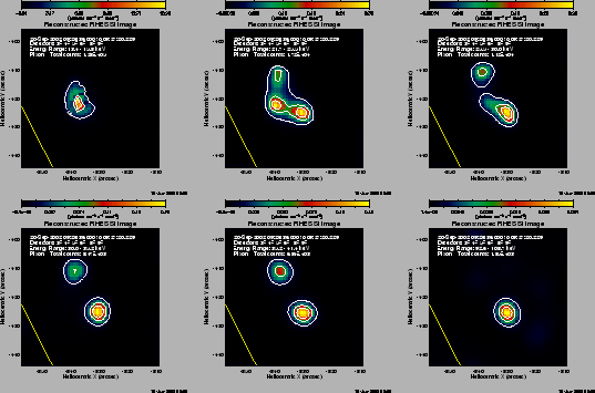Figure 3: Light curves of individual footpoint and loop-top sources in the 12-25 keV (left panel) and 25-50 keV (right) energy band for the 2092002 flare. The dot-dahsed, step-shaped curves show the ratio of flux of the two FPs to the LT sources, averaged over time intervals before, during, and after the peak. 'N FP' refers to the northern looptop, 'M FP' the middle footpoint, 'S LP' the southern footpoint. We note there are two distinct pulses in the 25-50 keV band. From the first pulse to the second, the LT emission is essentially constant in the 25-50 keV band but increases substantially in 12-25 keV. This suggests the LP spectrum undergoes softening, which may be explained by the evaporated chromospheric material dominating the LP emission.

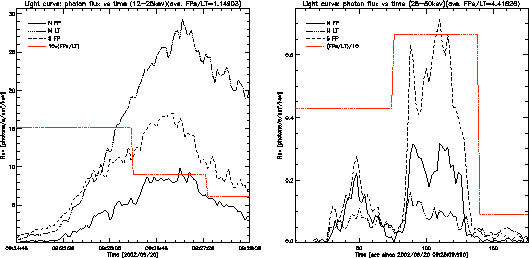Figure 4: Light curves (left) and source box definition (right) of the 2081203 flare.

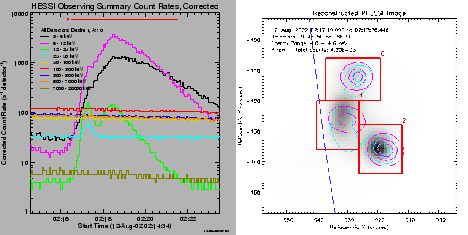Figure 5: PIXON images of the 2081203 flare at separate energies and times. The upper, middle and lower row corresponds to the rising, peak and decaying phase about the peak time, respectively. Energy goes higher from left to right columns. The temporal evolution indicates that: (i) in lower energy bands, the compact footpoints are the brightest sources in the rising and peak phase, but in the decay phase the looptop dominates and the emission tend to spread over the whole loop; (ii) in higher energy channels, the looptop ephemerally shines at the peak and rapidly dies away but the footpoints remain longer after the peak.

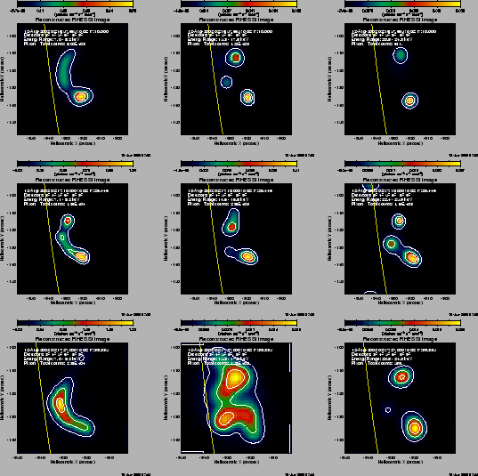Figure 6: Same as Fig. 3 for the 2081203 flare.

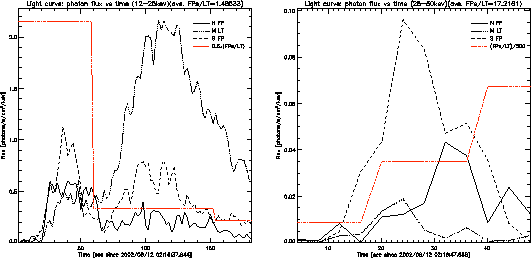Figure 7: Light curves (left) and source box definition (right) of the 2112532 flare.

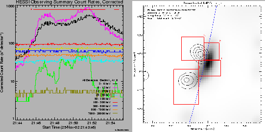Figure 8: RHESSI HXR images of the 2112532 flare.

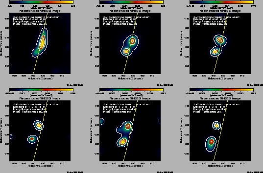Figure 9: Light curves of individual footpoint and loop-top sources for the 2112532 flare (same format as Fig. 3).

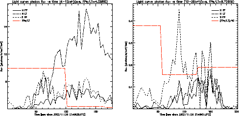Figure 10: Lightcurves of the 2080327 flare (left) and the source box definition (right). Contours and map are PIXON images at different energies. Two major flaring loops are identified, marked in thick, blue lines, and their corresponding looptop and footpoint sources are assigned a letter, A, B, C, etc.

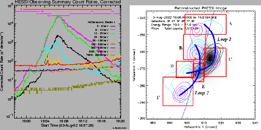Figure 11: RHESSI HXR contours (by PIXON) at different energies overplotted on TRACE 171 Å images for the 2080327 flare. Heliographic grids (dashed lines) have a $1^{\circ}$ spacing in both longitude and latitude. Note the TRACE images are at a later time which is best for one to see coronal loop structures in EUV. The TRACE images indicate that there are a series of magnetic loops and two of them are co-located with the RHESSI flaring sources (also see Fig. 10).

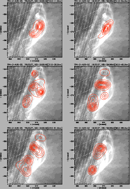Figure 12: Light curves of individual footpoint and looptop sources for the 2080327 flare (same format as Fig. 3). The upper panels are for loop 1 (refer to Fig. 10) in 12-25 keV (left) and 25-50 keV (right); the lower panels are for loop 2. It is interesting to note that the two loops do not contribute equally to the total emission: (i) in the 25-50 keV band, the total flux of loop 2 is higher in the first pulse but lower in the second than that of loop 1; (ii) in the 12-25 keV channel, the looptop of loop 2 is stronger than that of loop 1 by a factor of about 2 in the first pulse (although their total fluxes are comparable at this time) but much weaker by a factor of 4 in the second (loop 2's total flux is lower too). The looptop emission from loop 1 predominates over others in the second (major) peak in both energy channels. In the 25-50 keV band, the total flux of loop 1 (2) increases (decrease) from the first peak to the second. This suggests that the burst of loop 1 may be initiated by its interaction with loop 2. Please refer to the accompanying poster (# 18.03) by Jiang et al. for the spectroscopic characterists of the individual sources.

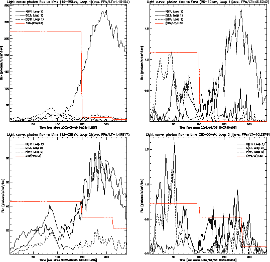Figure 13: Light curves (left) and images (others) at different energies of the 2082809 flare. In our PIXON images about the peak time, this flare appears as a single source on the limb in all the 13 energy bins from 10 to 54.2 keV. CLEAN images at different times also indicate a single source. The full spectrum yields a fit with a power law index of 5.0 and temperature 1.9 keV, suggesting this source is a looptop, presumably with its corresponding footpoints naturally occulted behind the limb.

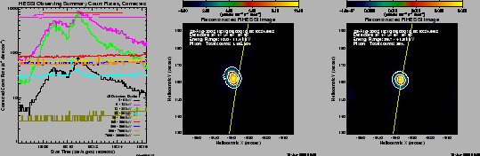Figure 14: Light curves (upper left panel) and images (others) at different energies of the 2111410 flare. From images, this flare does not show an appreciable looptop source possibly because the looptop is too faint to be detected (i.e., out the dynamic range) and/or the angular separation is not sufficient between the LP and FPs, considering its low heliocentric longitude of $71^{\circ}$, the lowest in this sample of the 22 flares.

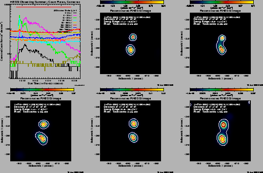Figure 15: Light curves of individual footpoint and loop-top sources for the 2111410 flare (same format as Fig. 3).

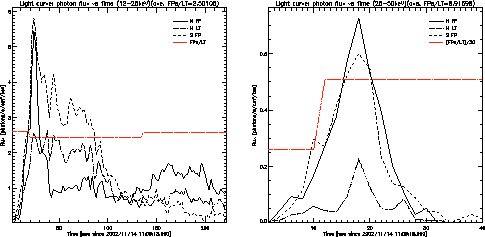Figure 16: The heliographic location distribution (left) and the histogram of the peak count rate (right) of the sample flares. The red vertical lines in the left panel marks $90^{\circ}$ in longitude (see Table 1).

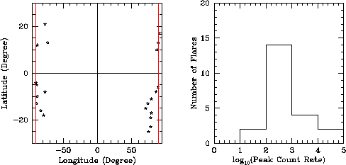Figure 17: Histograms of $R$, the FPs to LP flux ratios at different times and energies, with a bin size of 2. The upper cutoff is set at 16, about the upper limit of RHESSI images, and any ratio greater than this value is counted to the last bin (note this results in the tail bump at $R = 16$).

Miscellany

• Detector selection. For spectroscopic 'PIXON' images, the front segments of detectors 3, 4, 5, 6, 8, and 9 were used by default (with a few exceptions). Detector 2 was deselected for its threshold at about 25 keV and poor energy resolution of about 9 keV. Detector 7 was not included either because of its resolution of about 3 keV. We did not use detector 1 because its 2" spatial resolution is smaller than most of the smallest features in our sample. For lightcurve 'CLEAN' images, usually detector 3 through 8 were used.

• Background estimate. Since RHESSI is non-shielded spacecraft, the background in the data is high (Smith, 2002). There is no well-defined algorithm to subtract background for imaging at present. To roughly estimate the DC background in images, we simply selected a sufficiently large box to enclose all the major flaring sources. 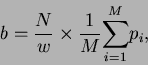Next we took the averaged pixel value in the image excluding the selected box as the background contribution to each pixel. For a boxed source with $N$ pixels, the background in the flux can be estimated as
  
  $$b = \frac{N}{w} \times \frac{1}{M}{\sum\limits_{i=1}^M}p_i,$$
  
  
  where $p_i$ is the individual pixel values (photons cm$^{-2}$ s$^{-1}$ arcsec$^{-2}$) in the image outside the selected box, $M$ is the number of pixels there, and $w$ is the width of the energy bin.

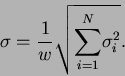
• Error estimate. The error estimate for RHESSI images is still a research program. Our first attempt was to use the 'hsi_calc_image_error.pro' routine in the Solar Software (SSW) IDL package to get the pixel by pixel error, $\sigma_i$, in an image. These errors are intended to give a measure of how well constrained each pixel is by the data given the image model derived from the reconstruction. The IDL routine determines how large a change in the image is required to make a one sigma change in the fit. The error for a source flux with $N$ pixels and energy bin width $w$ is
  
  $$\sigma = \frac {1}{w} \sqrt{ {\sum\limits_{i=1}^N}\sigma^2_i}.$$
  
  

Acknowledgments The work at Stanford is supported by NASA grants NAG5-12111, NAG5 11918-1. T. Metcalf would like to acknowledge support from grant NAS-98033-05/03. The authors would like to thank Dr. Kim Tolbert and Dr. Säm Krucker for their kind help with RHESSI software and data analysis.