 Figure 1
Using Green Function method suggested by Petrie and Neukirch (2000), we have computed 3D potential magnetic field, linear force-free field and non-force-free field from the light-of-sight magnetograms taken by SOHO/MDI; and using Boundary Element method ( Yan and Sakurai, 2000), we have calculated 3D non-linear force-free field from vector magnetograms taken at Beijing Observatory. Comparison of these results shows that (1) all models give similar and reasonable magnetic connectivity; (2) the pattern and twist of linear force-free field and non-force-free field strongly depend on the alpha while those of the non-linear force-free field are influenced by the transverse magnetic field; and (3) the height of non-force-free field lines is much higher than the other three's and the force lines are stretched vertically, agreeing with Perie and Neukirch's simulation (2000).
1.1 Models
potential field, linear force-free field, non-linear force-free field, and a non-force-free field model in which horizontal electric current component exists to balance plasma's pressure and gravity( Low, 1991 ).
1.2 Methods
Green Function method ( Perie and Neukirch, 2000) was used to compute potential field, linear force-free field and non-force-free field and Boundary Element method ( Yan and Sakurai, 2000) was used to calculatenon non-linear force-free field.
1.3 Boundary Condition
vertical magnetic field at the boundary surface was used as boundary condition in Green Function method while the vector magnetic field was used as boundary condition in Boundary Element method.
1.4 Data
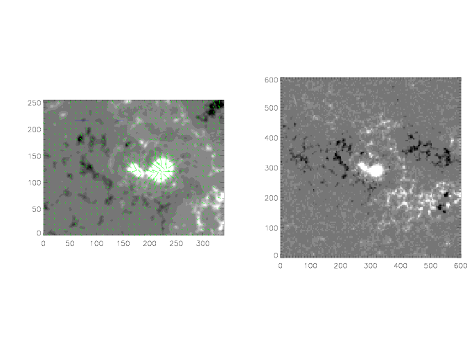
light-of-sight magnetograms taken by SOHO/MDI and vector magnetograms taken at Beijing Observatory (see Figure 1). We calculated the magnetic field in the active region NOAA8668.
A class of non-linear force-free fields in closed-form was proposed by Low and Lou (1990) and those fields provide vector field at the boundary surface from which extrapolation of magnetic field based on models mentioned above can be performed. A critical comparison can be therefore carried out to test the reliability and accuracy of those algorithms.
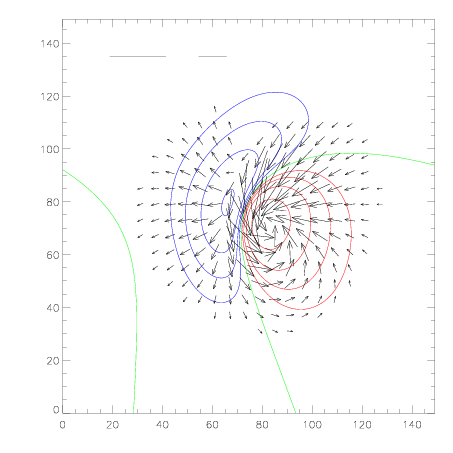
We take one of those solutions to generate magnetic field in the space and vector field at the surface boundary in order to perform the techniques for extrapolation. The magnetic field was generated by P_1,1 with l = 0.3 and FAI = PI / 2, where P_1,1 is the eigenfunction corresponding to eigenvalue a_1,1 = sqrt(0.425) (Low and Lou, 1990), l is the location of source point that is at (0,0,-l). The vector field is shown in Figure 01 where the contour represents longitudinal component with level of 20, 40, 80, 160 Gauss and the arrows are transverse component. The bars at the upper left are 100 and 200 Gauss.
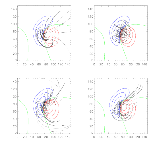
Figure 02 is the comparison of those models with the analytical solution. The top left panel is the analytical solution, and potential field, linear force-free field and non-linear force-free field are repsectively at top right, bottom left and right. The alpha chosen in the linear force-free field calculation is 0.05 unit ^-1, the best match by eyes to the analysical solution. Magnetic connectivity in those models appears similar and reasonable. Obviously, non-linear force-free field has better match with the solution in shape.
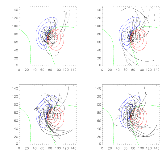
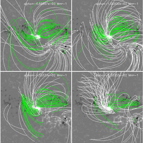
The structure of linear force-free field strongly depends on the alpha selected. The panels in Figure 03 show the linear force-free fields using variable alpha that are 0.02, 0.04, 0.06 and 0.08 respectively.
 Figure 3
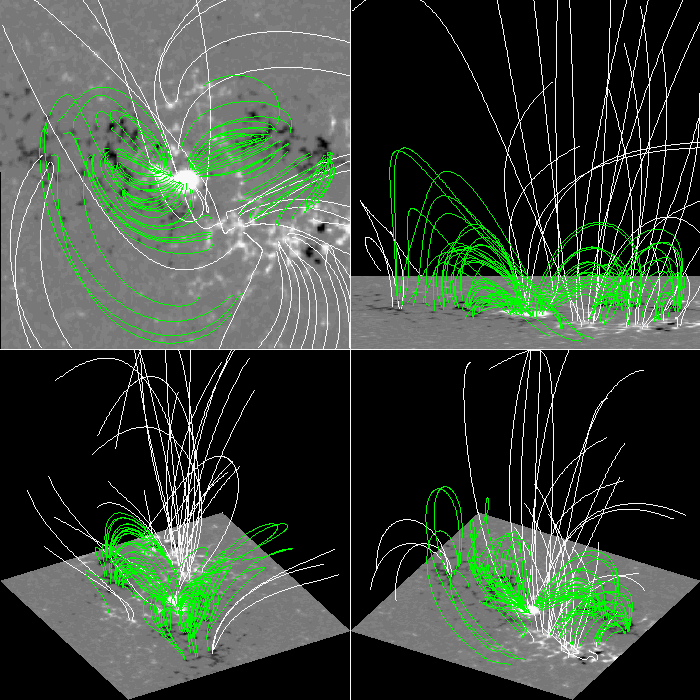 Figure 4
 Figure 5
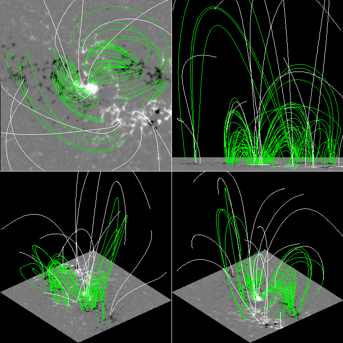 Figure 6
The fields on 19 August are calculated from the data shown in Figure 1. Figure 2 shows potential field (top left), linear force-free field (top right), non-linear force-free field (bottom left) and non-force-free field (bottom right) viewed from top, and the fields viewed from different sights are shown in Figure 3 (potential), Figure 4 (linear force-free), Figure 5 (non-linear force-free) and Figure 6 (non-force-free). The magnetic connectivity appears similar in these results and the height of non-force-free field lines is apparently higher than others -- the force lines are stretched vertically. Obvious twist is found in non-linear force-free field (Figure 5 ).
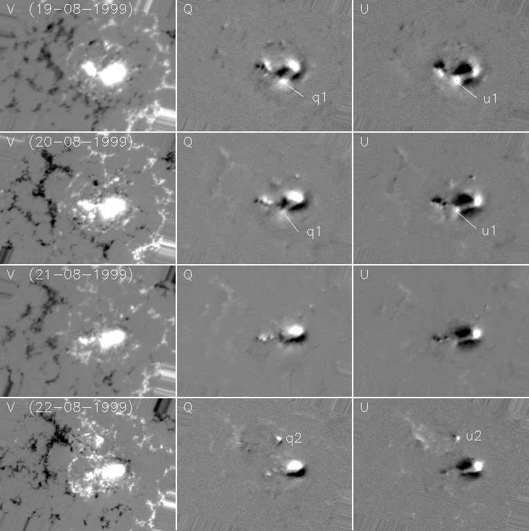 Figure 7
 Figure 8
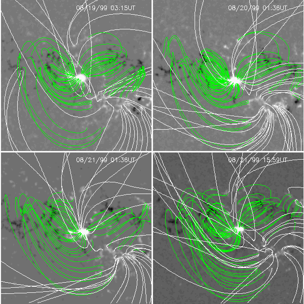 Figure 9
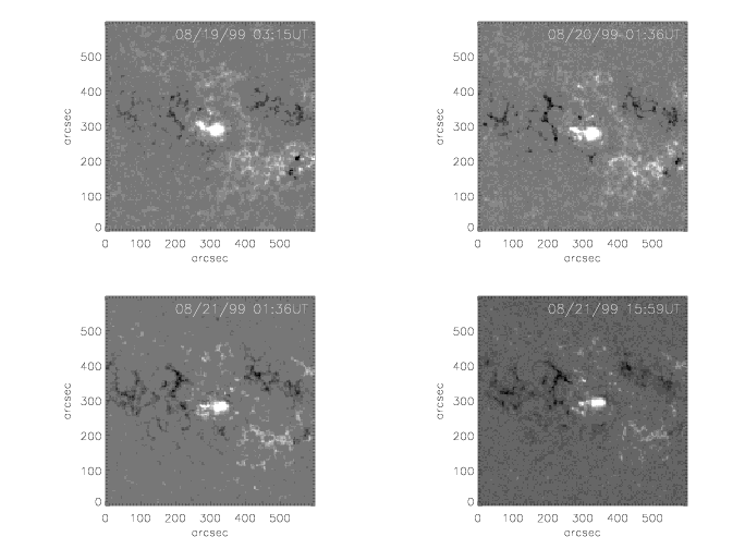 Figure 10
The change of the linear force-free field and the non-linear force-free field from 19 August to 22 August refects variation of the magnetic field on the surface. Decrease of the transverse magnetic component (q1 and u1 in Figure 7 where show Stokes map V, Q, and U in this period) causes the low-lying field system to turn out to be higher and eventually to be vertical ( Figure 8) while the emerging magnetic flux (q2 and u2 in Figure 7) is connected to negative patches that emerged simultaneously. The linear force-free field looks similar in this period (Figure 9) as light-of-sight magnetic component does not change evidently (Figure 10), except necessary magnetic connection is computed to connect the emerging magnetic flux. This indicates the magnetic connectivity inferred by calculation is reasonable. The alpha is chosen to be the same in these calculations.
While the pattern and twist of the non-linear force-free field are influenced by the transverse magnetic component on the surface, those of the linear force-free field are mainly controlled by the alpha (Figure 11). In this sense, the linear force-free field reproduced by this method is more uncertain.
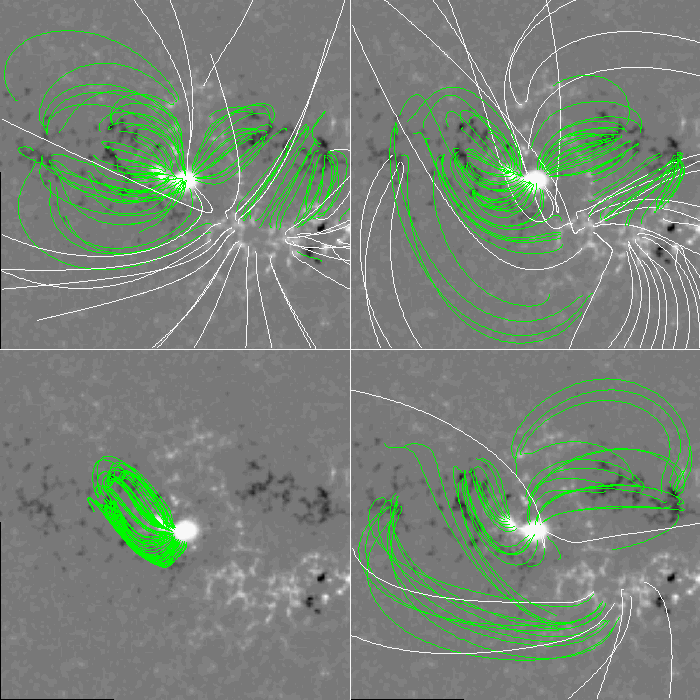
Comparison of these fields and observed SXT images shows part of bright loops and structure are well matched with the calculated force lines (Figure 12).
I.All models give similar and reasonable magnetic connectivity in AR8668, suggesting those methods are effective.
II. The pattern and twist of the field are influenced by transverse magnetic component and by chosen alpha in non-linear force-free field and linear force-free field respectively.
III. The height of the non-force-free field lines are much higher than the other three's and the force lines are stretched vertically that agrees with Perie and Neukirch's simulation.