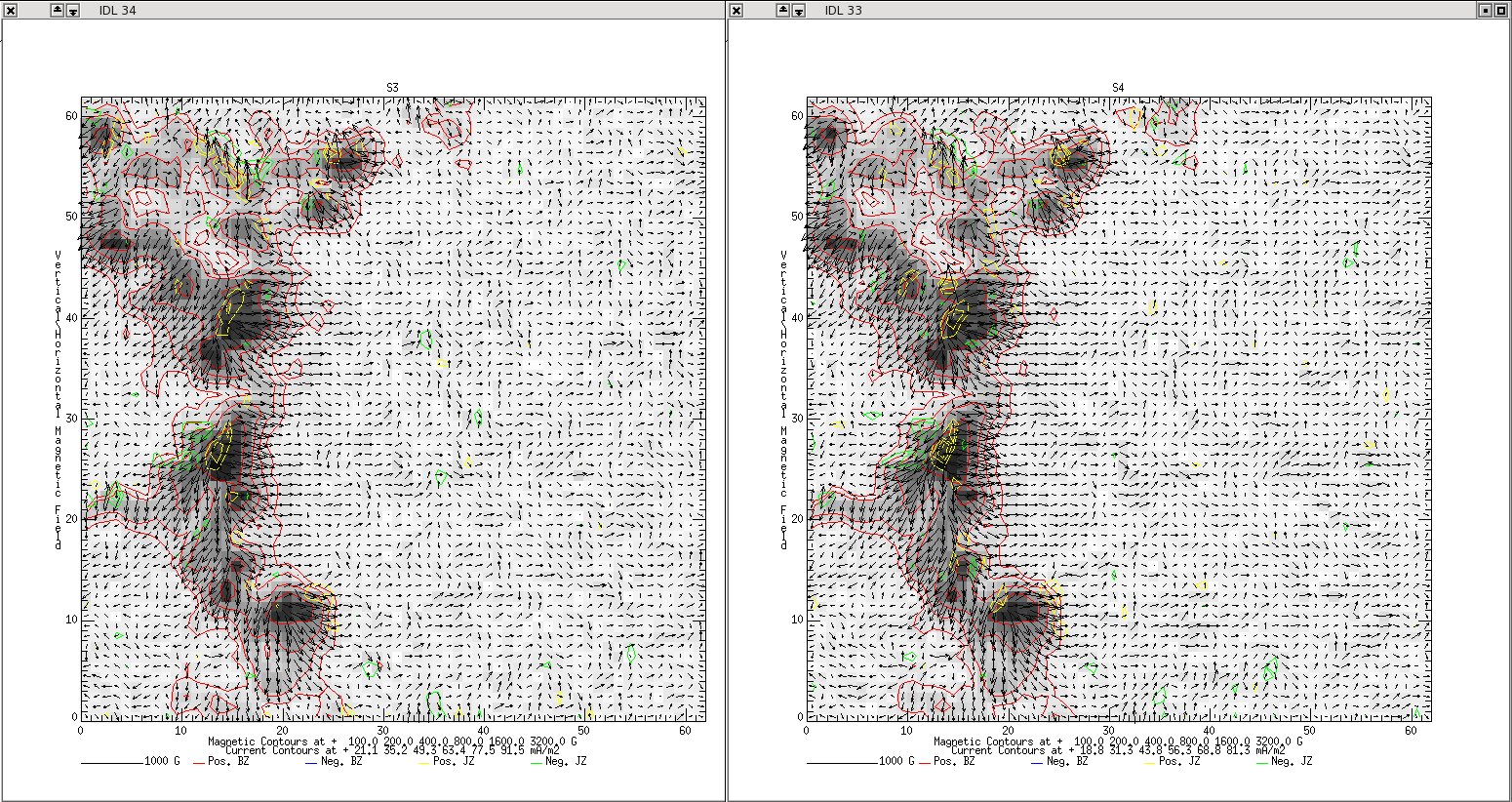
 S3 pdf file
 S4 pdf file
how to get hmi.S_720s: T_REC (definition), apodizing (description).
Summary: S5 is better than S3 and S4. Now use S5.
Now we are using S5. how to get S3, and correction done from S3 to S5 (Jesper?)
Definition of S3-5 (from Jesper)
S3. Spatially constant leakage (Q' = Q + q(x,y)I-->correct me if it's wrong). Time and spatial average.
S4. Spatially constant leakage plus PSF correction (Q' = Q + convol(I,ker)-->correct me if it's wrong). Averaged over time, but only center of disk.
S5. Radially dependent leakage (Q' = Q + q(r)I, and similar for U and V). Spatially constant PSF correction (disk center optimized). Both temporally averaged.
(from KD. on analysis on S3-S4)
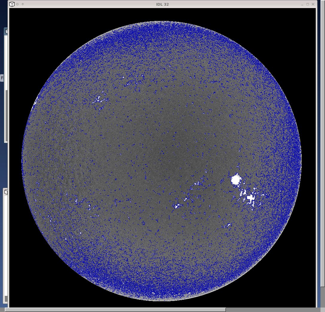
Comparing the files atan_dist_S3.ps (S3 pdf file) and atan_dist_S4.ps (S4 pdf file), the annuli sampled are the same and the color schemes are the same, but in this case, what is plotted is the distribution of a poor man's version of the azimuth, stepping through the wavelength positions as you step through the pages. Generally, as long as one does not cross strong fields, the goal is for these to be basically flat signifying an isotropic azimuthal angle distribution. You can see from the pictures of the annuli (in e.g., IQUV_dist_S3.ps) that the strong sunspot is missed, but that a couple of the annuli do cross some plage areas. It's also fairly clear that the distributions have basically become flatter, yet there is still some biased towards preferred direction.
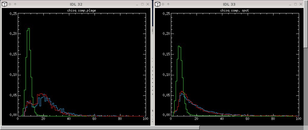
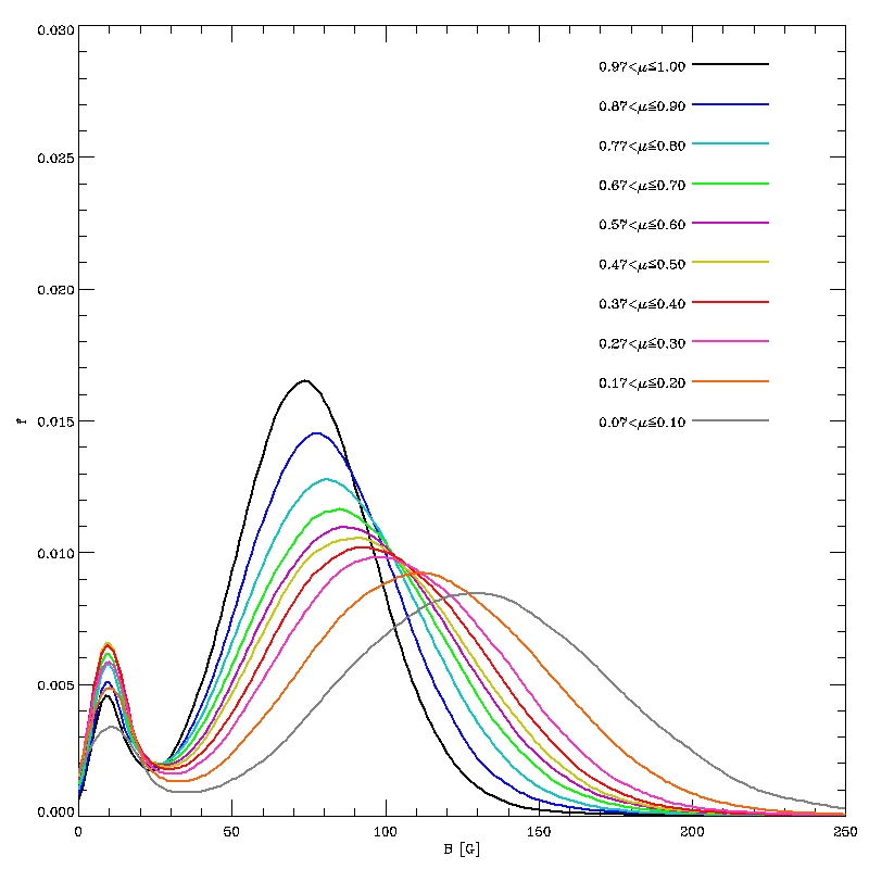
(from Jesper) What I did was to divide the images in 10 evenly spaced zones in radius, 0.0-0.1, 0.1-0.2, etc. The first two pages show the histograms with 4 degree bins in atan(U/Q)/2 (in the continuum, tuning position 0). Solid is S3 (spatially constant simple correction), dotted S4 (spatially constant PSF correction and implied optimization of the simple leaks for the center of the images and dashed S5 (radially dependent simple correction and spatially constant PSF correction).
As you can see the frequency 2 signal (presumed due to the PSF) is dramatically reduced from S3 to S4, as expected. Not much change in that from S4 to S5.
The frequency 1 signal (presumed due to the simple crosstalk) is more complicated.
To look at things in more detailed I fitted sine waves with 1 and 2 periods (over 180 degrees) to the histogram using a FFT. Results are on the next two pages. As you can see the frequency 1 component became smaller near the center and larger further out when going from S3 to S4. This makes sense since S3 was based on a spatial average and S4 effectively on disk center. Adding a radial dependence to make S5 resulted in smaller amplitudes than for S3 and S4 at almost all radii. Not sure if the small worsening around 0.7 is a statistical fluke, activity or because the correction is based on a temporal average.
As expected the frequency 2 component drops dramatically when the PSF correction is introduced. For whatever reason there is also a small improvement going from S4 to S5 away from disk center.
I don't know how much of the residual variations in S5 are due to each of temporal variations, spatial variations in the PSF, statistical fluctuations and so forth. I may try estimating some of these.
Further tests: What I did was to custom made PSF corrections for the target image. These are the various line and symbol styles:
Solid: S3. Spatially constant leakage. Time and spatial average.
Dotted: S4. Spatially constant leakage plus PSF correction. Averaged over time, but only center of disk.
Dashed: S5. Radially dependent leakage. Spatially constant PSF correction (disk center optimized). Both temporally averaged.
Dash-dot: Radially dependent leakage from temporal average. PSF from center of target image.
Squares: Same, but spatial average of PSF correction.
Plusses: Radially dependent leakage from temporal average. Linear spatial dependence of PSF correction.
Diamonds. As the plusses but also has radially dependent PSF correction.
Given the changes made the last plot (frequency 2) is probably the one to concentrate on.
First of all you can see that using the actual PSF correction for the center (dash-dot) improves the results at the center. Not surprising.
The spatially averaged correction (squares) gives a modest improvement over much of the solar image.
There are also some improvements when including the spatially dependent PSF correction.
Summary: Range +-0.648A is bit too narrow to include the sidelobes.
Regarding the ongoing discussion about the filter transmission profiles in vfisv.
To calculate these profiles, we are currently using 49 wavelength points, from -0.648 A to +0.648 A, with a separation of 27 mA. The range, [-0.648,+0.648] A (around the Fe I line wavelength) is too small.
For the 6 filters, there are significant sidelobes outside this range. Here is the part in the integral value of each filter that the sidelobes outside the [-0.648,+0.648] A range contribute to (for the pixel (2048,2048)):
for I0: 9.21%; I1: 6.42%; I2: 5.44%; I3: 6.22%; I4: 8.14%; I5: 11.40%
This might be an issue since these numbers vary from filter to filter. They also vary slightly from pixel position to pixel position on the CCD (the filter profiles have a spatial dependence). Here is how the integral value of the filters in vfisv compare to the integral value of the filters calculated on a fine wavelength grid over a large range (using the int_tabulated function of idl, and for the pixel (2048,2048)):
hi-res filters vfisv filters
I0: 0.046249973 0.041440750
I1: 0.046278311 0.043538356
I2: 0.046275892 0.043299675
I3: 0.046242405 0.043154288
I4: 0.046185737 0.042464215
I5: 0.046108407 0.040240574
as you can see, the integral value of the filter transmission profiles has a relative peak-to-peak variation of 8.2% in vfisv (meaning the filter I4 is assumed to transmit 8.2% less light than I1), while the actual relative peak-to-peak variation is only about 0.4% (I4 and I1 transmit pretty much the same amount of light).
I don't know the exact impact this has on your inversion of the Stokes parameters, but it most likely introduces some errors somewhere. I understand that you cannot use a fine wavelength grid over a large range because of speed constraints, but maybe you should use more points than just 49?
I calculated the filter profiles using a phase map of the end of March 2010, and then using a phase map of end of November 2010 (the last one before retuning). This way we can see the impact of the drift in the Michelsons on the filter profiles (the retuning reset this drift). This is the maximum impact we are likely to ever have: we plan to retune HMI every 6 months, so the maximum Michelson drift should always be less than what is considered here by comparing March with end of November.
The result is in attachment to this email. The black solid line shows a filter profile (for the filter I0) calculated on a fine grid, using the phase maps of March. The red symbols show the profile calculated by vfisv, also with the phase map of March: you will notice that the 2 sidelobes at +0.85 and -1.15 A are completely ignored by vfisv (and there are other smaller sidelobes further away). The orange symbols show the filters obtained with the phase map of November. So, indeed, because of the Michelson drift, using a phasemap from March to process observables data in November will result in an error. However, it seems to me that this error is smaller than the one you make by ignoring significant sidelobes outside of the [-0.648,+0.648] A range.
I could modify the routines in vfisv that compute the filter profiles, so that it takes in account the dates of the data you want to process, and fetch for a phasemap closer in time (not sure how to access DRMS functions from inside vfisv.c: it does not look like a DRMS module. I guess you are using a wrapper or something?). Or do something simpler: we know by how much the Michelson drifts, so depending of the dates of the data, I could correct the phases of the Michelsons (it would have to take into account retunings though). However, it seems to me that the error you make on the filter profiles by using an old phasemap might not be as large as the error you make by using only 49 points over a very limited wavelength range. I would suggest you first increase the wavelength range.
Summary: fill factor = 1; no stray light.
fill factor is set to be 1 everywhere now. (Borrero: "Fitting for the filling factor at all times can cause problems where the polarization level is low. From tests I had made with Hinode, VFISV has this problem in about 1-2 % of the pixels.");
stray light profile hasn't been applied to; (Duvall: "The bottom line is that in a moderate-sized sunspot that the observed in the center of the umbra might be contaminated by 25% scattered light.")
Test is done with the original initial guess settings and new settings (Dopper velocity is used as initial guess for vlos_mag--Fig.e-6; and Dopplergram and Blos are used as initial guess--Fig. e-8). Module settings are, for fig. e-6, weighting=1,3,3,2, stop criteria=e-6, dopplergram as initial guess, maximum iteration=200; for fig. e-8, weighting=1,3,3,2; stop criteria=e-8, dopplergram and magnetogram as initial guess, maximum iteration = 200. The results are different.
Summary: two schemes are proposed. One (1-3-3-2) probably works better in sunspots and
the other (1-7-7-3) seems working better in quiet Sun.
- When I compared the inversion results for the magnetic field inside of strong field areas (sunspot) I saw that the new Voigt function produced more abrupt discontinuities in the field strength than before (of the order of 200-300 Gauss). They were present before, but were not so large.
- In order to remove these discontinuities I started changing the chi2-stop requirement for smaller values, but it didn't seem to make any difference inside the sunspot. It's only effect was that it reduced the number of inclination spikes outside of the active region.
- Then I went on to modify the weights towards more uniform values for I, Q, U, V. I started at the usual 1-7-7-3 and ended up in 1-2-2-2. I saw improvement throughout the tests (in the sense that the discontinuities in the sunspot started washing out), but towards very low values other issued begun to appear.
- I settled on 1-3-3-2 and ran a full disk inversion. The lower weights work better in the sunspot but worse in the Quiet Sun. Making the convergence criteria more strict, you can improve the 'spike issue' in the QS but convergence will also take somewhat longer. So we have to decide where we put our threshold.
More tests on weight schemes and convergence-stop criteria
Trying to think about what is going on here. The scenario I think I have forming is something like: unweight I -> easier to get into problems due to Doppler shifts but takes Q,U,V into account better for 'better' (smoother-looking) sunspot solutions. Weight I stronger and thermodynamics and shifts are better constrained but polarization signal is not utilized. In Quiet Sun, weight Q,U,V more, tends to reduce the spikes in the inclination of the magnetic field, making it tend to 90 degrees, and consequently yielding larger field strength values. This happens more so as we go towards the limb. In sunspots, giving more weight to Q,U,V, unbalances the solution because the absorption in I is small, that it becomes "unimportant" in the chi2.
We're concentrating on V_dop, but recall that the greater correlation with field strength would probably be doppler width or eta_0. But those will be very sensitive to what it believes line-center to be. (Q:remind me in VFISV, is V_dop from I or from V-crossing? A: From both. We invert the four Stokes parameters simultaneously. I guess it depends on which one dominates and how they are weighted relative to each other.)
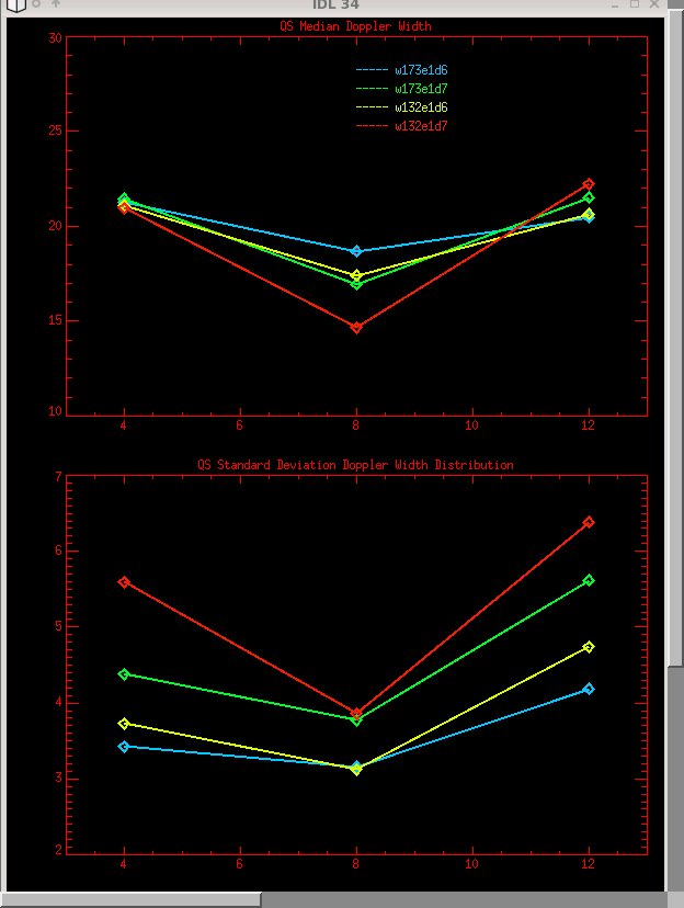
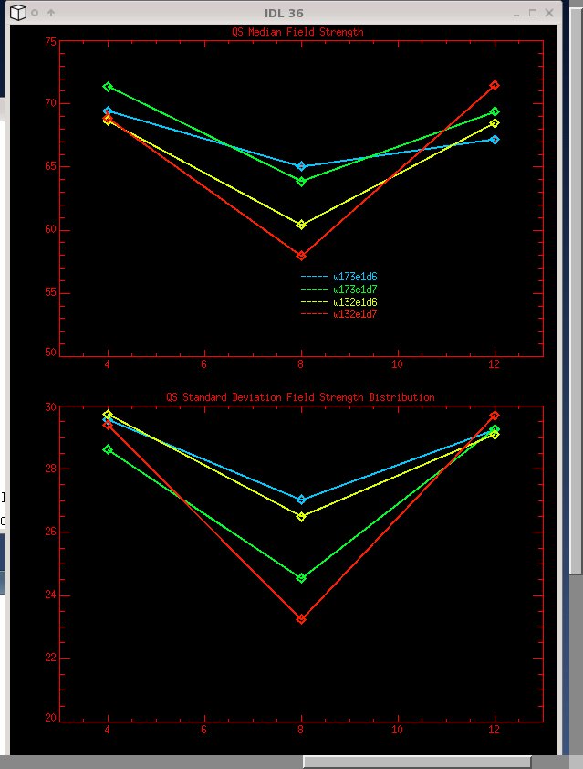
The figures below show temporal variation of the inversion results with the different weight schemes and convergence-stop criteria. The data are from a quiet region. Y-axis is time in hour.
Thus two weight schemes are suggested. One (1-7-7-3) appears to work better on quiet Sun, in the sense we saw less spatial variation of inverted data over the whole disk, but the data (total strength) in sunspot (especially in umbrae) shows obvious discontinuity. The other (1-3-3-2) works better for sunspots: that discontinuity is minimized greatly. But there are large-scale variations over the disk in the total field strength data. [One solution (from Todd) is to process the data with the latter scheme at a regular basis (12-minute cadence), and with the former scheme in a much lower cadence such as 6-hours or 12-hours.] But it's for one time only. It did *not* minimize the discontinuities at other times, so we need to decide on a weighting scheme that behaves overall the best for a full orbit's worth of data, both for quiet-sun (minimize variations) and sunspot areas (minimize discontinuities).
Summary: No clear evidence shows that stricter convergence-stop criteria (e-7 or e-8) do a
better job than e-6. Low-signal pixels may contaminate possible trend. need further test.
Three convergence-stop criteria have been tested (e-6, e-7 and e-8). Specifically, the thought is that if it is converging well, then there should be little difference in the solutions between e-6 and e-7. But the differences were not small. testing e-8: if differences are small between it and e-7, great. if still large, bigger problems loom.
Plotted here is the median of field strength in an area of 1024x1024 at disk center as a function of time. Basically no active regions are in this area. Same stats done for chi2. From one weight set to another, the chi2 shows big differences, mainly due to a normalization issue. From one convergence criteria to the next, chi2 doesn't change much at all, which means there is no significant overall improvement in the fits just because we force the code to go up to the maximum number of iterations. But for a reason that I still don't understand, we give the code the opportunity to favor some parameters with respect to others when it can iterate indefinitely.
One thing I think is really important is to understand what is happening with the stopping criterion, irrespective of the weights and the temporal variation. Has the inversion actually found a minimum in chi squared or not? If not, what is it doing?
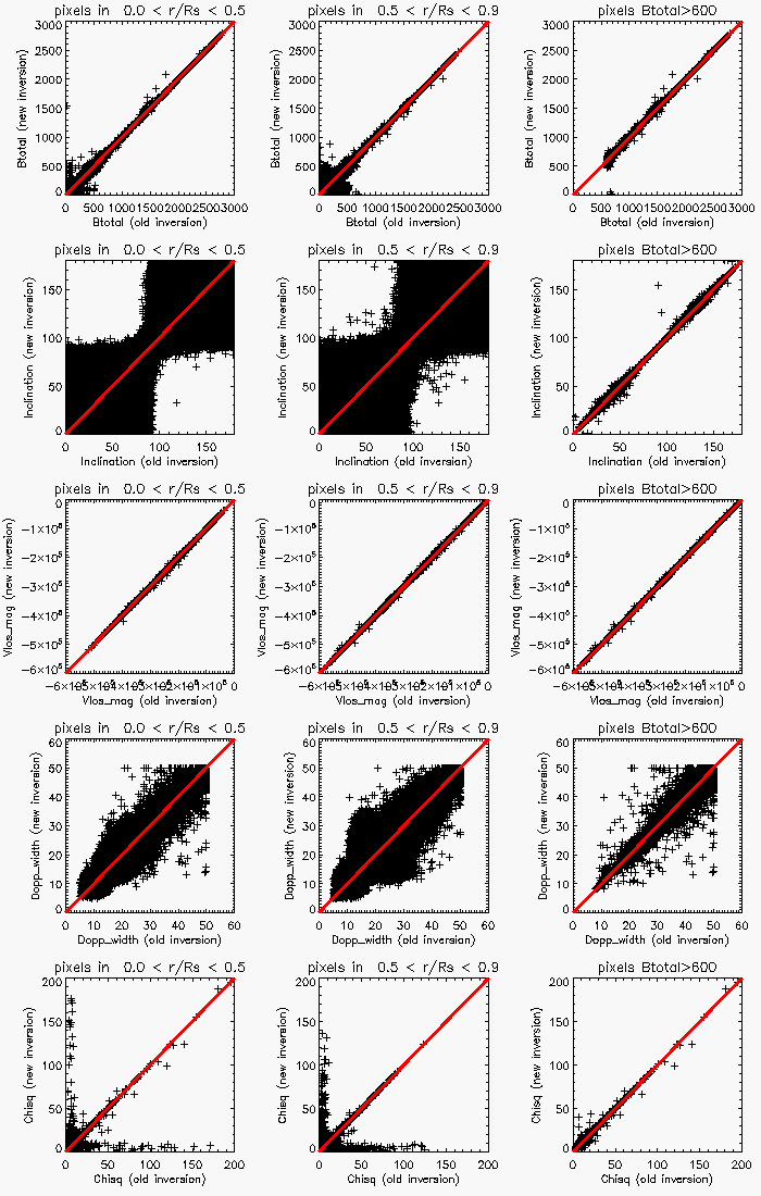
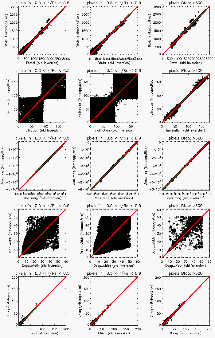
To do this, it would help to know what changes as the value of epsilon for the stopping condition is made smaller. For a single time and a single set of weights, would you please make scatter plots of the Doppler width with one value of epsilon versus the Doppler width with a different value of epsilon, and maybe do the same thing for the field strength, since those are two of the fit parameters we've been looking at, and do the same thing for chi squared.
But for sunspot, especially for strong field, the scatter is greatly minimized. First page of the pdf file (all data pdf file) corresponds to w = [1,3,3,2], second page to w=[1,5,5,3] and third page w=[1,7,7,3]. The fourth page shows the same as the first one, but for pixels that have B > 600 Gauss only. The scatter almost disappears when only strong magnetic fields are considered. I think that we can conclude that for larger field strengths we don't have nearly as much ambiguity between parameters and results don't change depending on the convergence criteria and number of iterations, right? (Could the fill factor constraint explain any of the Doppler width sensitivity?)
 all data pdf file
 sunspot only pdf file
On tracking the evolution of chi2 for several pixels throughout 200 iterations. It was very useful to see what is happening in individual pixels to understand how the optimization is working.
There are 4 figures (corresponding to 4 different pixels) that show the evolution of chi2 and the magnetic field strength as a function of the iteration number. The first 3 figures correspond to disk center quiet Sun pixels, and the last one to a sunspot. The convergence criteria was set to 1d-12 to force all pixels to go to 200 iterations. The red vertical lines correspond to the places where the code kicks the model parameters randomly because there have been too many consecutive iterations where chi2 has increased.
I have a few thoughts and questions on what you sent out, but I do think it was very useful to see what is happening in individual pixels to understand how the optimization is working.
First question: were these pixels chosen because they showed large changes in field strength and doppler width when the stopping criterion was changed? Or were these just some "typical" pixels?
It seems that the inversion fairly consistently does a random perturbation about every 20 iterations. In the documentation I have for VSIFV, it says that the condition for a random perturbation is an increase in chi-squared for too many consecutive iterations (currently set at 6). Is this still the condition?
I would really like to understand why this was chosen as a condition for a random perturbation. As I understand the LM method, if chi-squared increases, then the parameter lambda (using the notation of Numerical Recipes) is increased, and the code attempts a step with the new value of lambda. Most of the time, adjusting the value of lambda should (eventually) result in a step which reduces chi-squared. One exception to this is if the code has already found the minimum, in which case a step in any direction can only increase chi-squared. It sounds like the way the code is set up now, rather than stopping at the minimum, it would randomly perturb the minimum and start again, which doesn't make much sense.
The reason I see for a random perturbation is to let the code try again if it has fallen into the wrong local minimum. When the value of chi-squared is properly normalized, this can be checked by looking at whether the chi-squared at the minimum which has been found is (much) greater than 1. If it is, then it's probably not the global minimum. Although it's still not formally correct, you could try what Pete suggested a week or so ago and "Normalize the weights so that they sum to 1? This way the may be interpreted "loosely" as model probability." This might give us an idea of whether the optimization has found the correct minimum or not.
I do not have a lot of intuition for how the LM method behaves, but if you think that the 6 consecutive increases in chi-squared is not a result of the code finding a minimum, then I would suggest that increasing the number of changes to lambda before a random reset would be a good idea. Someone correct me if I'm wrong, but it seems to me that if the code has not actually found a minimum, and it's not in a particularly pathological part of parameter space, then there should be some value of lambda for which it can take a step which decreases chi-squared. I would think it is preferable to keep going to the minimum it's in, rather than randomly starting somewhere else in parameter space.
{(from Graham): Is this the complete list of possible stopping conditions for the inversion now? If so, I am not particularly surprised at what you found about how many pixels have a flag of 2. Since the chi2 is not normalized in a standard statistical sense, picking a single value of epsilon as a stopping condition is not going to work well for all pixels.
I believe there are several other fairly standard stopping conditions for an optimization code like this, such as looking at the rate at which the parameter values are changing (if they are changing slowly, then the code is likely to be close to a minimum), and looking at the rate at which chi2 itself is changing. I thought Rebecca had been experimenting with some of these other conditions. Is that true? If not, I think they might be helpful in determining which pixels have converged properly to a minimum.
Right now the code checks for the evolution of chi2. If it starts converging too slowly, then it will stop iterating and exit the procedure succesfully. Also, the epsilon value that checks the rate of convergence depends on the continuum intensity, so it's not a fixed value for all pixels. The last version of the documentation reflects this properly. What you're quoting belongs to a previous version, sorry. The maximum number of iterations is set in the wrapper to 30, if I remember correctly.
When the evolution of chi2 is satisfying (= in the good direction) but too slow, we assume we're getting very close to convergence, so we stop the iterative process and exit the loop with a success flag (flag = 0). Whatever the value of chi2 is, if the evolution is still fast enough, the code won't exit the iteration loop. It will only exit the loop when chi2 doesn't seem to improve at a decent rate.
I guess then I don't understand then why you have an epsilon value which is dependent on the continuum intensity. I think the standard approach is to look for a small fractional change in the value of chi2, so when change in chi2 is less than epsilon times value of chi2. This should not require a varying epsilon. Does the code presently check the magnitude of the change in chi2?
Yes, the code checks how big the change in chi2 is. However, since chi2 is smaller towards the limbs, small changes are still significantly big in terms of the fits. When I was doing these tests I found that I had to account for the continuum intensity so that the evaluation of the change of chi2 was "fair" to all pixels. Same argument for sunspots.}
so far, no.
Summary: Larger maximum number reduces the un-convergence pixels greatly. Now it
is set 200.
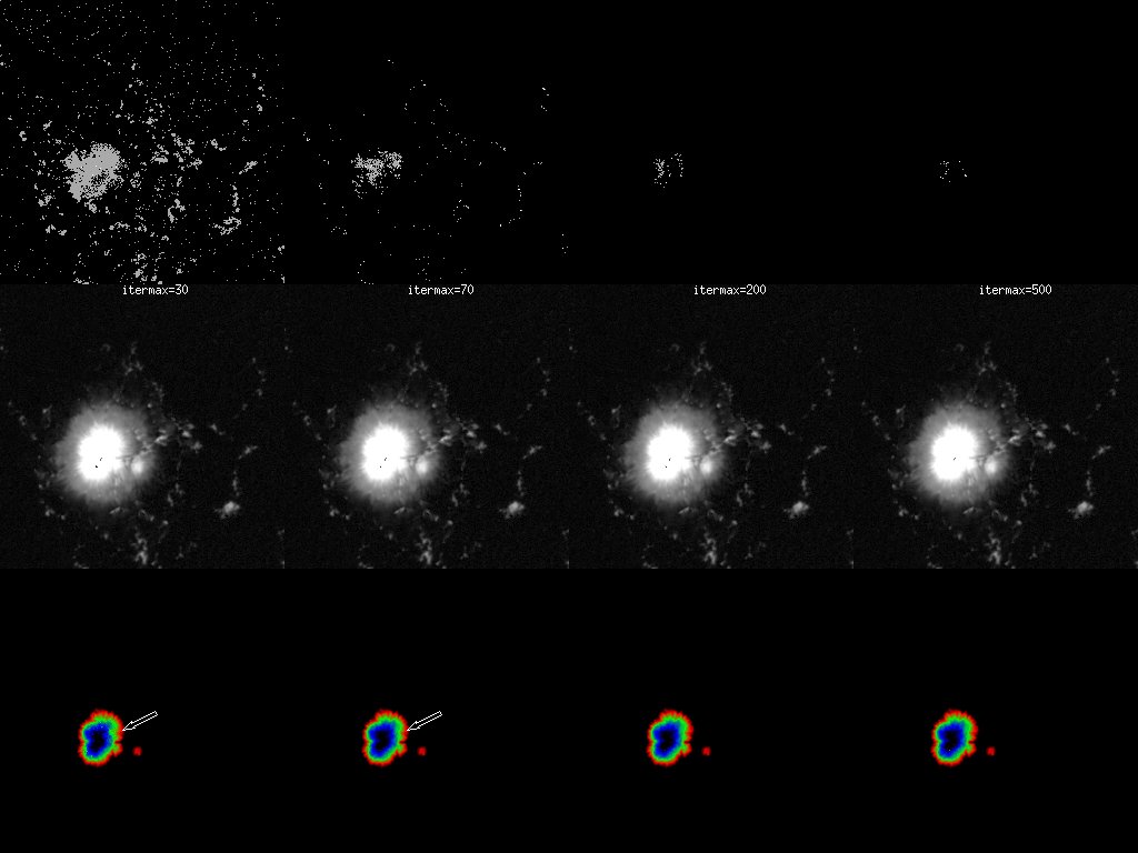
I've taken a quick look at the azim_flg_strng_incl_alot.fits file that Keiji produced (which provides azimuth, convergence flag, field strength, and inclination for runs with maximum iterations set at 30, 50, 70, 100, 200, 300, and 500.)
In short, the number of points which transition from a convergence flag of 2 to a convergence flag of 0 decreases dramatically with increasing maximum iterations. There is some indication that the resulting solutions (with an increased maximum iteration) are better, meaning that they are more consistent with their neighbors and consistent against additional changes in maximum iteration limits. This is true for the plage area as well as the sunspot itself.
Attached are some plots, which I'll explain in a minute. I do want to remind everyone that just because a convergence flag of zero is returned, it does not mean that we are necessarily in the right global minimum, or that the solution is in fact correct.
itermax_effects1.jpeg (effects1 file): top to bottom is the convergence flag image, field strength scaled 500:3000, and field strength scaled 1500:2500, with a weird color table and an arrow pointing to a region of interest. Going across as labeled are the iteration maxima. The top row shows that the number of pixels labeled as "converged" increases quite a bit, and that the non-convergence flags were not limited to only the sunspot with the maximum of 30. The middle row shows that without looking carefully, one may infer is that there is very little difference between the results from the different maxima. The area highlighted by the arrow in the bottom row is where the convergence of flags were nonzero, even though the area to one's eye looks "basically OK". But in fact, it "smooths out" substantially (and convergence -> 0) with a higher maximum.
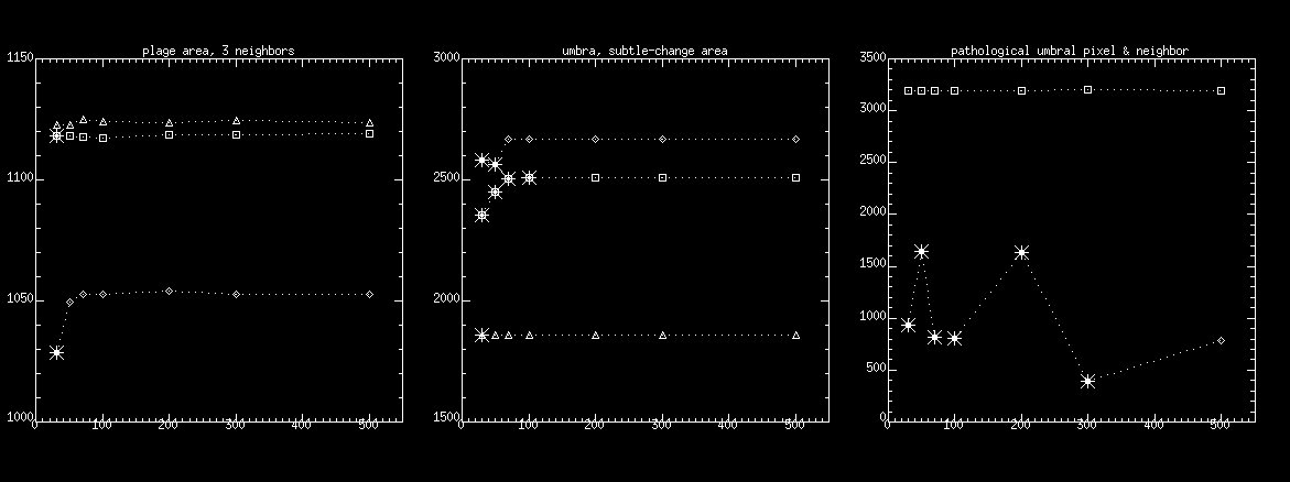
itermax_effects2.jpeg (effect2 file): plots from a couple of points as labeled showing field strength as a function of iteration maximum. For all, those points with non-zero convergence of flags have large asterisks. Left panel are three neighboring plage area points, middle are three points in the area of that subtle change indicated by the arrow in the previous plot, and the right panel is a comparison of one of the umbral pathological pixels and its neighbor.
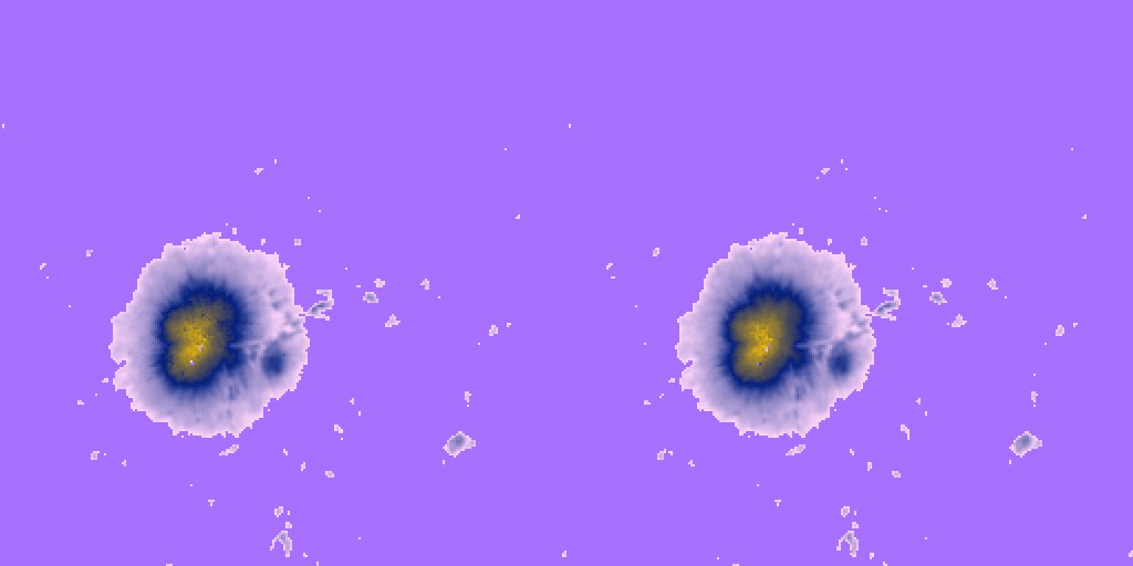
itermax_effects3.jpeg (effects file): It is saturated and such to highlight the difference between a max of 30 (left) and max of 300 (right) in the "smoothness" of the sunspot area solutions.
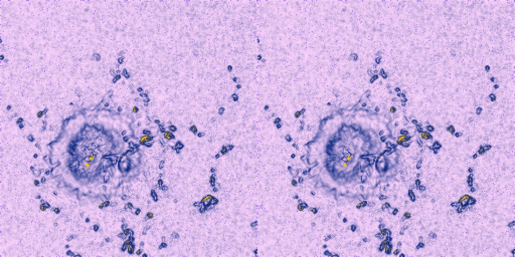
itermax_effects4.jpeg (effect4 file): the local spatial gradient of the previous image, which highlights the somewhat subtle, but I think important indications of a solution which is at least more spatially consistent using a larger number of maximum iterations.
Bottom line: without embarking on a research project on optimization methods or much more additional work on refining the stopping conditions themselves, I would suggest increasing be iteration limit to at least 100, preferably more like 200.
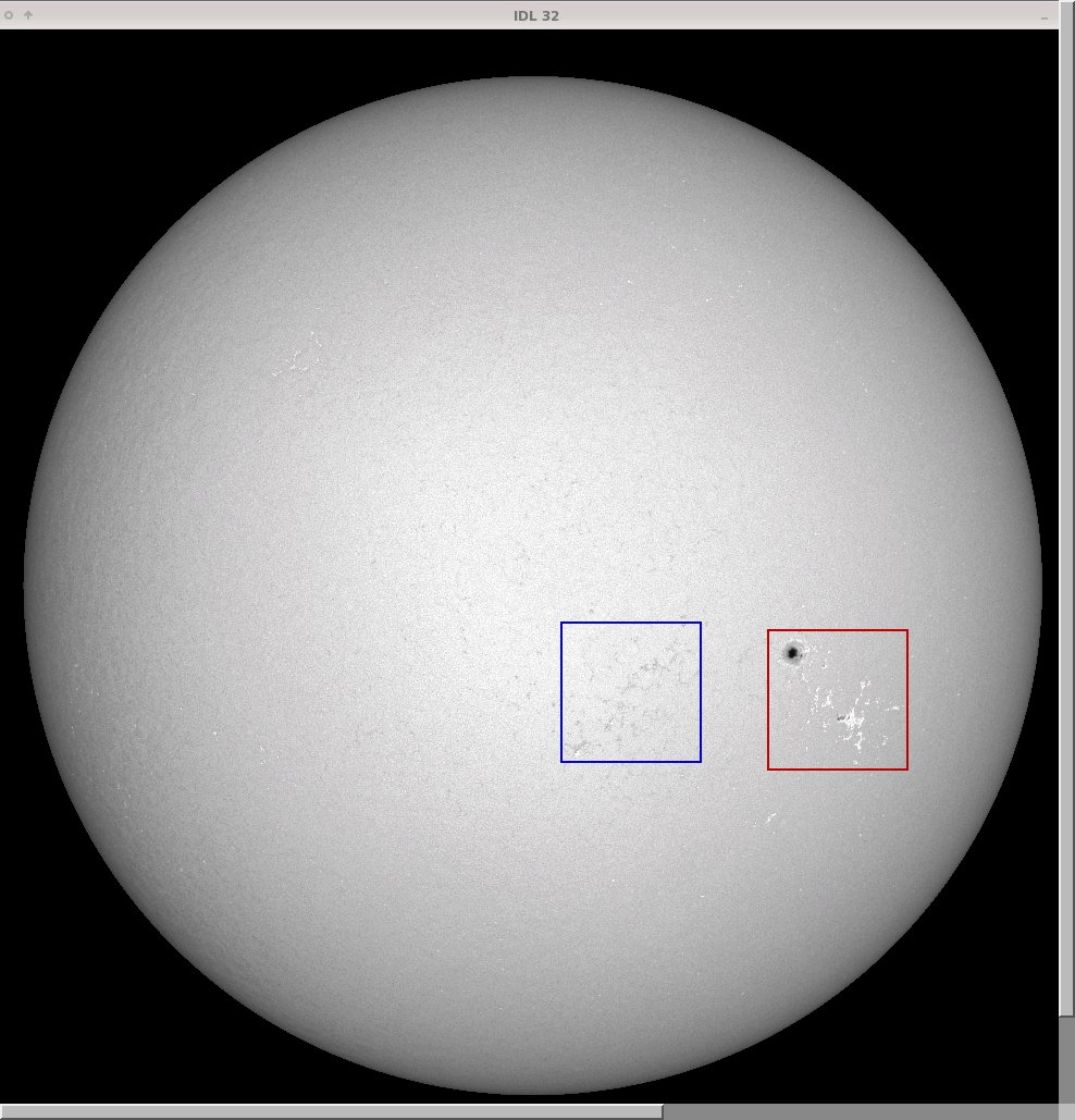
subareas.jpeg (subarea file): image is actually the source function constant (for no good reason but that I had it loaded), blue and red boxes show sub areas that I looked at, in part because I wanted to look not only at the sunspot area but at the quiet/plage areas. both the subareas are 512^2.
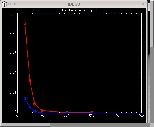
frac_unconverged.jpeg (unconverged file): as the names suggests, the fraction of the pixels within each sub area ( blue: plage, red: spot) which have a nonzero convergence flag, as a function of maximum iteration. Interestingly, the plage area has predominantly convergence flag of zero, and the nonzero areas are predominantly pixels that do have some polarization signal.
next, within the plage subarea, I mapped out the points that had either the combination of B>500 and conv=0 (at itermax=30) or B>500 and conv.ne.0 (at itermax=30). picked a couple at random, and confirmed that the kind of changes visible in the sunspot area (with respect to itermax) are also visible in these weaker areas, and also in the thermodynamic parameters in addition to the magnetic parameters. so:
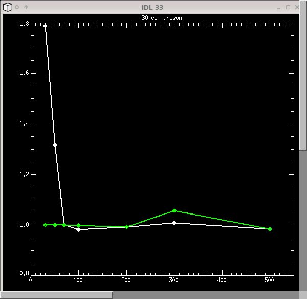
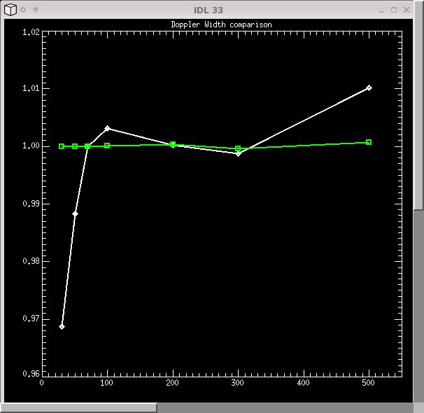
dopp_width_comparison.jpeg and B0_comparison.jpeg (B0 = constant term of the source function): comparison of two points as described above, percentage change with itermax, i.e. the parameter is normalized by the value that it obtains when it first converges, green:conv=0 (at itermax=30), white: conv.ne.0 (at itermax=30).
there is nothing profound here, except to reiterate that it's not just the field parameters that are affected by non-convergence, they all play into and around each other, and reiterating that at least with the uncertainties and chi-squared calculated incorrectly (we hope), an itermax of 200 will improve not only to spot areas, but the solution's stability for the rest of the full disc as well.
 subarea file
 unconvergence file
 B0 file
 doppler width file
And also the comparison of chi-squared values. Two subregions as before (see titles), within each: green is the chi-squared distribution for FLAG = 0 pixels (normalized their total number, usually about 250,000) for itermax = 30. Blue; chi-squared distribution for FLAG ne 0 pixels at itermax = 30; Red: *same* pixels, final chisq for itermax = 500.
Results: (a) while points which have difficulty converging do generally have "worse fits" (insert all caveats about proper normalization of chi-squared here), not all do. but it could be a good start (b) the chi-squared measure is not changing significantly even after lots of iterations, yet we have seen from other comparisons that the solution does become at least more stable within its part of parameter space.
Summary: need further check to make sure it's reasonable.
I've run 96 realizations of the inversion of a patch of quiet Sun at disk center, adding to the actual Stokes data in the patch some random noise (based on the estimations by Jesper and Sebastien for the 12-min averages). So for each pixel in the patch (100x100 px) I get 96 different results for the magnetic field strength, inclination, azimuth and so on.
In an attempt to understand the deviations caused by photon noise, I subtracted the average result from the 96 individual realizations (for each of the 10000 pixels in the patch) and did some scatter plots of these differences.
The square root of the variance of the azimuth is of the order of 50, and definitely always less than 180. Given that the azimuths are probably the most random quantity (in quiet Sun areas), I'm not surprised that the variances are large within the maximum range of uncertainty. I agree that the behaviour of the variances of the azimuths are weird, but it might have to do with the fact that there is a modulation in the PDFs of the retrieved when the input is noise (this is just a wild guess). Also the 180 degree ambiguity will be most obvious at the ends of the [0,180] range.
I changed the noise level in the wrapper to 50 (it was set at 150). We still propagate only one value of sigma to the chi2 for all of the Stokes parameters instead of one for the intensity and a different one for Q, U and V (it doesn't matter that much, because if I change the sigma for the intensity, I would have to compensate it by changing the weight too, so to keep the sensitivity of chi2 to all of the parameters).
The Hessian and divergence matrices were defined as negative. The signs canceled out when calculating the solution to the system of equations, but I changed them anyway, just for consistency.
With comparison between the Monte-Carlo and inversion.
[Jesper comments: Regarding the input noise I still think that it would be better to have different ones for different variables and change the weights as needed.
Also, it sounds like the noise is constant? Again I would prefer to scale it with sqrt(I) (with a corresponding change in epsilon). Of course that supposes photon noise. As we saw from the chisq it appears that there is more going on. If it is p-modes instead the scaling would have to be different.]
Summary: Large wavelength coverage of filter profiles gives a
result different with the narrow coverage; more samplings need updated result.
Originally, we were doing +/-0.648 Angstroems from the spectral line center, with a spectral sampling of 27mA. This neglects some contribution from the wings of the HMI filter profiles. I'm running tests over the Oct 15 datasets with +/-1, +/-2 and +/-3 Angstroems from the center of the spectral line with the same spectral sampling (27 mA).
I chose the weights and convergence criteria that yielded the strongest variation in the quiet Sun field strength across the disk as a testbed for this: weights = [1,3,3,2] and chi2_stop = 1d-7.
top: original inversion with +/- 0.648 A coverage
bottom left: +/- 1 Angst.
bottom right: +/- 2 Angst.
The plot on the second page shows a horizontal cut through these last two.
According to Sebastien, the relative error in the integral of the filters when the range is restricted to: a) +/- 0.648 A is of 7.4% b) +/- 1 A is of 5.0% c) +/- 2 A is of 1.48% d) +/- 3 A is of 0.68%
I can appreciate an improvement in the flatness of the result across the disk as the wavelength coverage is increased. On the right is another run with the full coverage of filter profiles (+- 2A). Initial settings are 1-3-3-2 of weightings, e-6 of convergence-stop criteria, and 200 of maximum iteration. The temporal variation is minimized.
One of the issues that we've been talking about was how large a wavelength coverage do we need in the synthesis in order to account for the outer lobes of the filter profiles properly. We run some tests with +/-1 A, +/-2A and +/-3A at either side of the center of the spectral line (as opposed to the +/-0.648 A that we had been using until then). We found out that the wavelength range made a difference, which was substantial from 1 to 2 A coverage, but minimal from 2 to 3.
Keiji and I worked on a hack to the code to account for an extended wavelength coverage without having to do the forward modeling in the full spectral range. I ran a test for a +/-2A spectral coverage case, using both the hacked and non-hacked versions of the code. The test was done on a 400x400 pixel patch on 2011.03.09 data. The non-hacked uses 149 spectral points at a 27 mA sampling and does the forward modeling for all of them. The hacked version uses 149 spectral points at a 27 mA sampling, but does the forward modeling for a central region with a width of 49 spectral points. For the remaining 100 points (50 at either side of the inner spectral range), we integrate the filters and multiply them by the model's continuum.
In this pdf file there are some more detailed explanations and some plots of the differences between certain quantities calculated in the two ways. The differences are of the order of 0.1% or less in the retrieved thermodynamical quantities. There is a slight difference in the average chi2 obtained from both methods, but I think that overall, the "hack" does the job pretty well.
Test run is done for more wavelength samplings for 8 and 10 filters. The large-scale spatial variation is still clearly seen.
Summary: No dramatic change is found in the inversion data due to
tuning change.
The change in tuning happened between 2010.12.13_19:47:25.21_UTC and 2010.12.13_19:47:27.10_UTC.
Bottom line: I don't see any large, dramatic systematic changes with the tuning in the field parameters for strong field areas or for the weak areas, aside from something consistent with that expected w/r/t doppler-velocity.
Summary:
720s versus 5760s
I had a quick look at the inversion of one of the 96-min averages. It appears that the noise in the field strength has decreased by at most a factor of two, which probably isn't enough to conclude anything much more than we could from the 12-min averages.
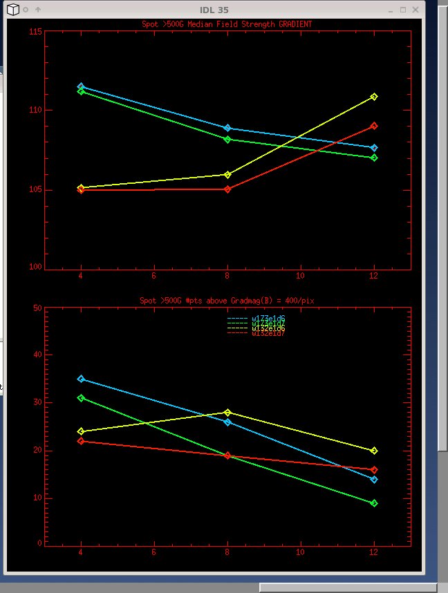
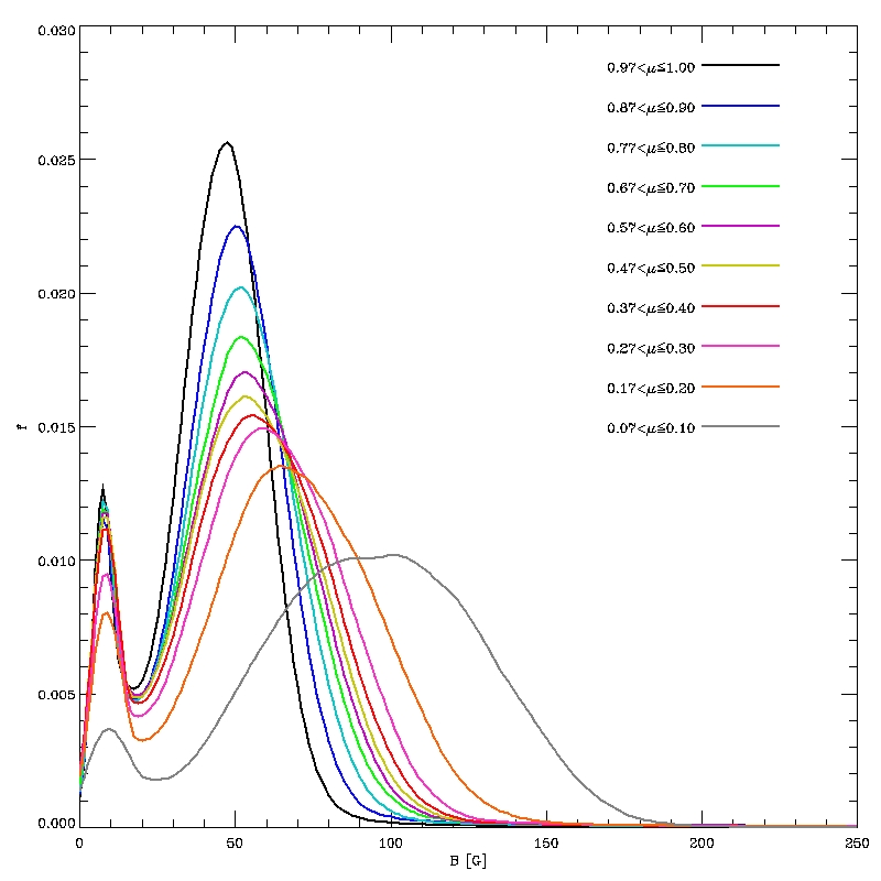
The attached jpegs show the distribution of the field strength in annuli of approximately constant distance from disk center, for the new 96-min average, and for an old 12-min average (so the inversion may not be exactly the same between these two) for 2010.10.24_00:00:00_TAI. The peak of the distributions should roughly estimate the detection threshold for the field strength. For the one closest to and including disk center (the black curve), the peak occurs at around 70G for the 12-min average, and at around 45G for the 96-min average. For annuli further from disk center, the peaks move to stronger field strengths, as expected, but the ratio between the 12-min average and the 96-min average doesn't appear to change much.
Summary: 24-hour and 12-hour periodicities are found in inversion data, as well
as in line-of-sight magnetograms from both cameras. They are likely related to the orbital speed. A 6-hour
periodicity is likely in the inverted field thrength data. Don't know what causes it.
24-hour and 12-hour periodicities are seen in the inversion data (as well as in the line-of-sight magnetograms from both cameras). Obviousely, it's due to the orbital velocity. The inverted field strength for one active region seems to suggest another 6-hour periodic behavior.
Plotted here is the median of field strength in an area of 1024x1024 at disk center as a function of time. Basically no active regions are in this area.
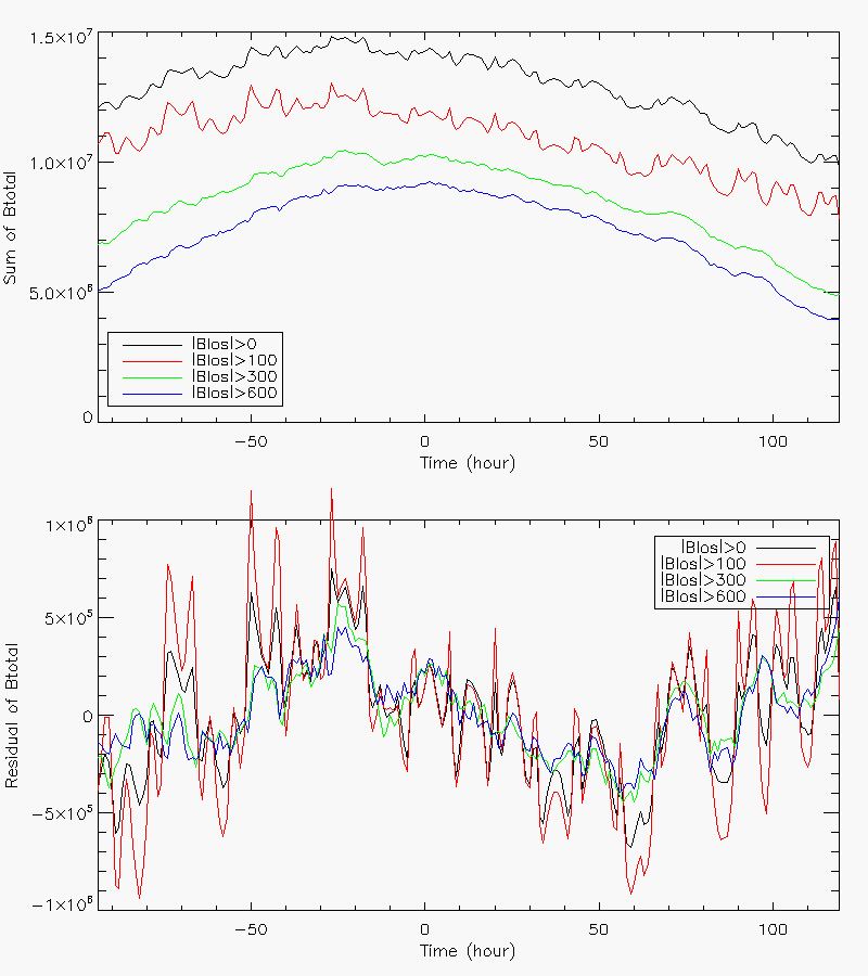
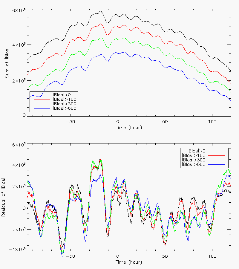
The field strength (from inversion) of an active region also shows periodicity. Data are from hmi.ME_720s for an area of 240*240 pixel^2 enclosed the active region AR11092 from July 30 to August 07 (240 hours in total). The curves in the top panels are sum of the field strength over this area from the pixels with a line-of-sight field greater than 0.0 (black), 100.0 (red), 300.0 (green), and 600.0 (blue). In the bottom panels are the residuals of the sum from a 2-order polynormial fitting to the data. There are roughly 35 peaks (by counting the red curve) in this time interval, which gives a 6.1-hour period. The maximum change is about 10% (estimated from the red curve).
Line-of-sight field also shows such periodicity. Data are from hmi.M_45s (left panels) and hmi.M_720s (right panels) for the active region AR11092 from July. 30 to Aug. 07. The region On July. 30 was at x=[3500, 3500 + 240], y=[1600, 1600 + 240]. Curves in the top panels are sum of the |Blos| over an area of 240*240 (pixel^2) from the pixels that have a field greater than 0.0 (black), 100.0 (red), 300.0 (green), and 600.0 (blue). In the bottom panels are the residuals of the sum from a 2-order polynormial fitting to the data. 24-hour periodicity is obvious. 12-hour periodicity is visible. 6-hour periodic pattern is not appreciated. The amplitude can be more than 10%.
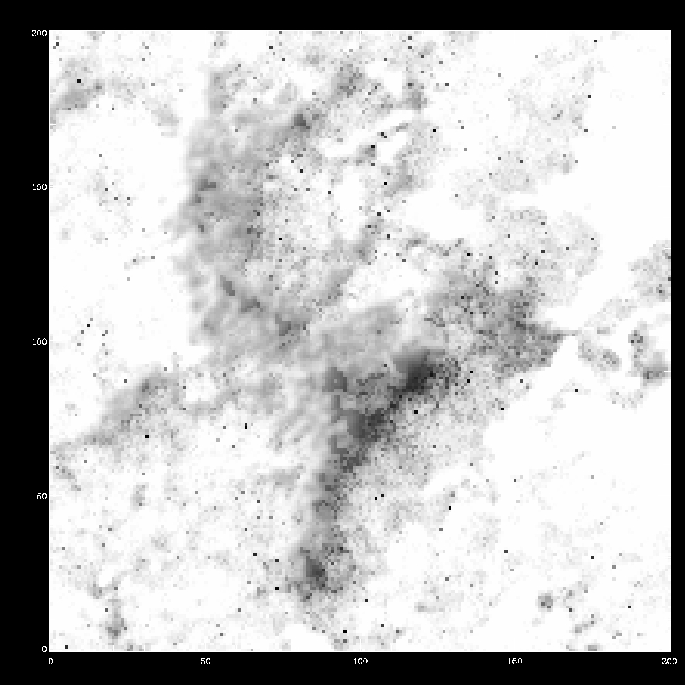
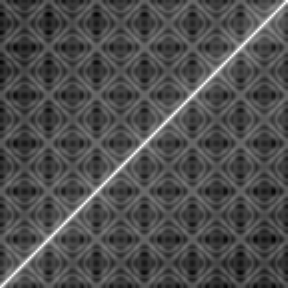
Cross correlation between pairs of field strength image. The pixel (i, j) shows the cross-correlation between the ith and the jth image in the 144-image series. Field is saturated at 150G to minimize the effects of active regions. The cross-correlation typically varies from 0.94 to 0.98. The diagnal lines show a 24-hour period. Some other periods are visible too. (how to do the plot: The images are first rebinned using the IDL rebin function and then scaled linearly from 0 to 150, by IDL bytscl function. They are scaled alike. The cross-correlation images uses a linear scale as well. You can get the original numbers in the fits file in that directory. The 144 scaled magnetic field images are also there. Anyways the difference in correlate ranges from 0.94 to 0.98. Not sure if that's significant.)
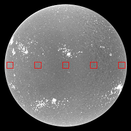
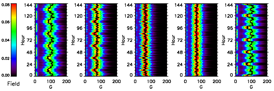
tacked histograms of field strength within 5 cutouts. The bins are 5G wide. Color indicates the normalized occurance in each bin. The black line denotes the bin with the largest occurance (beside the peak near 0). Daily variation is clearly visible on the limbs, with a 12-hour phase offset between the limbs. Disk center seems to display a combination of the modes from the limbs.
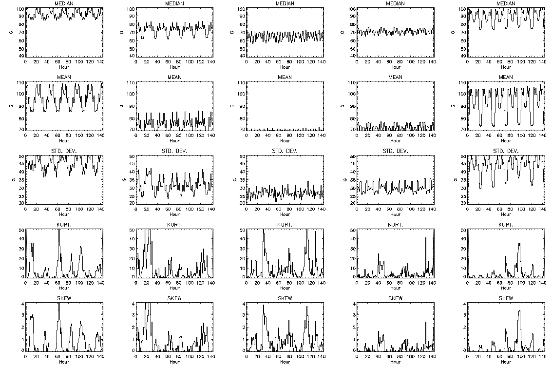
6-day series of median, mean, standard deviation, kurtosis and skewness of each patch. The leftmost plots are for the East limb, and so on. Again, both 24-hour and 12-hour variations are seen on the limbs, and they are out of phase by 12 hours.
Interpretation for 12-hour and 24-hour periodicities:
The tile pattern: Let us assume that the artifacts vary as the radial velocity of the observer. This, of course, means that you will see large correlations at lags of multiples of 24h, thereby explaining the +45 degree lines spaced by 24h.
Now, let T0 be the time of the maximum radial velocity and let the observing time be T=T0+dT. Which times then have the same velocity? Obviously T'=T+n*24h, for integer n. But also the one at T'=T0-dT+n*24h=T-2dT+n*24h, thus explaining the -45 degree sloping lines.
Why the artifacts are there to begin with: Sebastien has pretty much explained that. Even if you resolved the filters well, you will still suffer from the inaccuracies in our knowledge. For the Doppler velocity and LOS this has been largely corrected, but not for other variables. Try looking at the the mean of the line depth with time. Probably not surprising that this would lead to changes in the field parameters. Hard to know if it works quantitatively, though.
Comment: I agree with Sebastien that even if the filter profiles are not known exactly, we need to use as much information as possible with respect to the inversion. I think that with the orbital line-shifts, the asymmetric side-lobes could easily (if subtly) change the line shape. This sets the stage for the rest of the magnetic parameter determination. And the coarse wavelength sampling for the filter profile...I don't recall the details of that, but given these issues, it doesn't sound good. We need to at least start with +/-2A, and sampled as finely as needed to not lose information.
I think that the periodicities they see in the inverted full vector magnetic field is just do to the filter transmission profiles they use in the vfisv code. These profiles are not correct because: 1) we do not know the filter profiles with a good enough precision. there seem to be residual errors at the 1% level 2) in vfisv, to speed up the calculations, they use a very coarse wavelength grid for the filter profiles, and their wavelength range is too limited Therefore, the filter profiles used in vfisv are incorrect, which translate into 24h periodicities when the orbital velocity of SDO moves the average central wavelength of the Fe I line back and forth...
In the los observables code, I apply a lookup-up table correction on Vlcp and Vrcp before calculating Vdoppler and Blos. I also apply the polynomial coefficient correction (Vdrift) to both Vlcp and Vrcp before calculating Vdoppler and Blos. However, the linedepth and linewidth are uncorrected, and the continuum intensity is only partially corrected (only Vlcp and Vrcp used to calculate Ic are corrected, but not the linewidth and linedepth).
Wonder if where the field is strong, the lookup table correction is like a signed correction which cancels when added and doubles when subtracted. How big is the signal.
Summary: Large-scale variation is seen in inversion data. not sure what causes it:
background velocity? filter profiles? ...
The dynamic range of SDO is +/-6.5 km/s. Large-scale variation is seen in inversion data.
These trends are seen primarily in weak-field/week-signal areas, but the fact that they are strongly visible in thermodynamic parameters usually implicates something systematically changing with the line shape; obviously we expect line shape changes from center to limb, but east/west limb differences I would not expect, (except as influenced by the combination of various Doppler velocities combining in nasty ways with the wavelength sampling, hence the inversion code having systematically fewer points to fit, for example, on one limb versus the other..).
Details: bb.jpeg (Btotal file) is scaled 0--200, contours at 100, mostly for effect/emphasis of large-scale trends. doppwidth scaled 10--50, eta0 scaled 5-20.
 Btotal file
 eta0 file
 Doppler width file
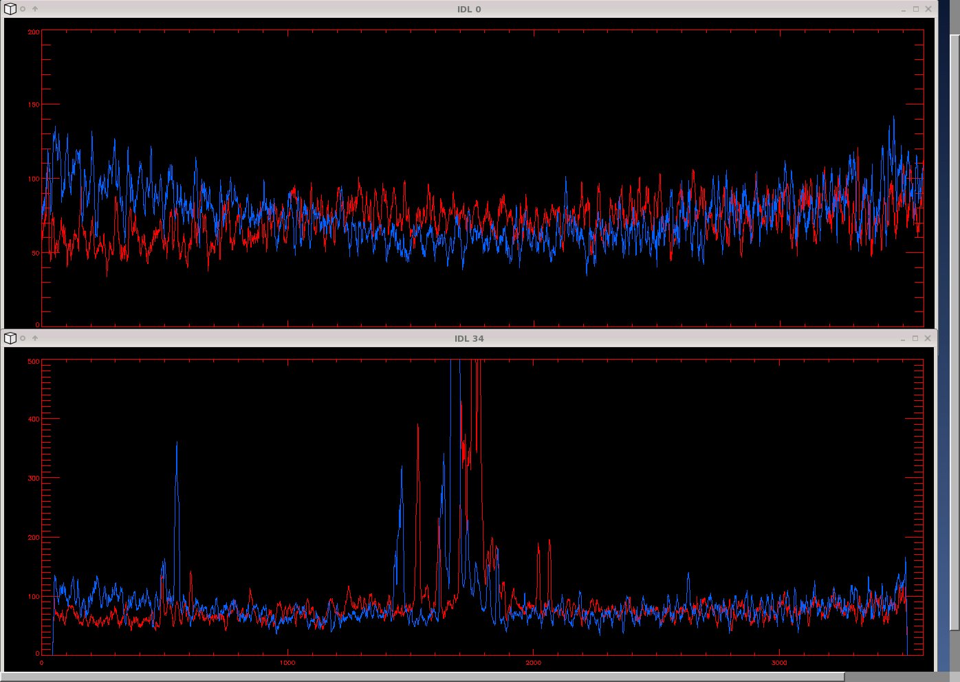
21Febcomp2.jpeg (comp2 file) : slices (**smoothed by a factor of boxcar of 10!**) (top) across the middle of the disk, yrange=[0,200] and (bottom) at y=2840, yran=[0,500] red: 15 oct 00:00, blue: 04:00. 4 hr different. The latter is closer to what I'd expect, and we checked - all quality flags are 0 for these data.
But a 100 Mx/cm^2 difference is more than photon noise. And that's about the level of these temporal/spatial variations.
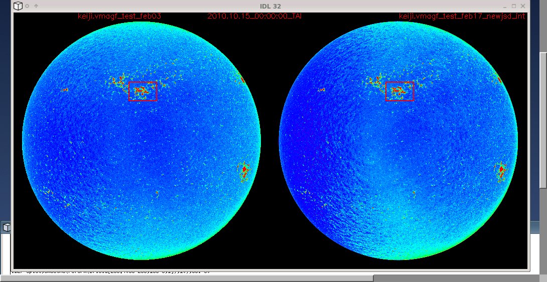
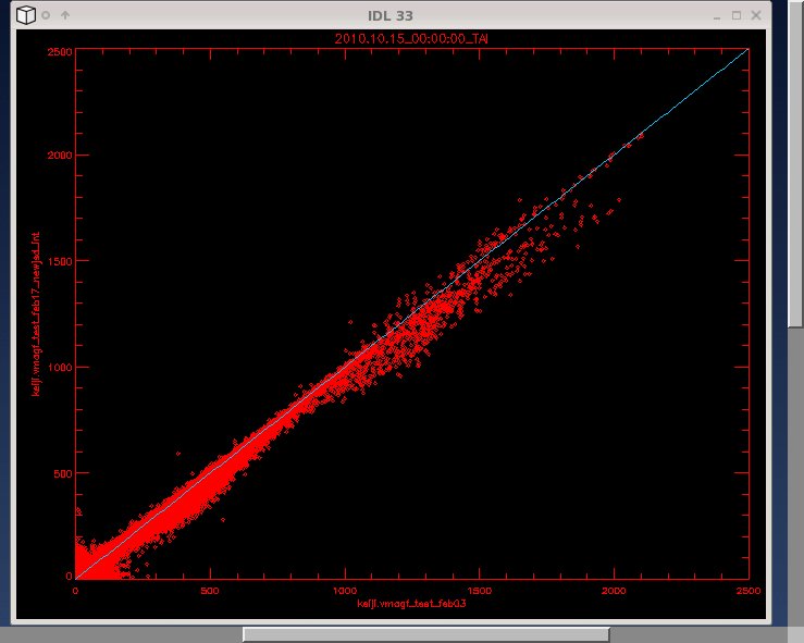
21Febcomp3.jpeg (comp3 file): 15 Oct 00:00, left/right the old/new series (keiji.vmagf_test_feb03/(keiji.vmagf_test_feb17_newjsd_int). What all changed between these I'm not sure I can keep track of. voigt-function error, #iterations? weights? filter profiles used? Someone please check because the newer ones are, qualitatively, worse in that there is a greater large-scale variation than before, in a pattern that I don't expect and in a manner that I'd not expect from changes to the inversion per se.
21Febcomp4.jpeg (comp4 file): scatter plot of field strengths within that small box indicated in 21Febcomp3.jpeg. New series (y-axis) systemmatically smaller field strength than old series, (x-axis).
Summary: Generally in quiet Sun. due to low signal?
I chose a small field of view around disk center. I inverted it with the standard set of weights (1, 7, 7, 3). Then I substituted Q, U and V of the same data for random noise that tried to follow the actual distribution in the Stokes profiles, and run the inversion again, with the same sets of weights.
Observations:
- The spikes appear in the synthetic random data.
- The distribution of inclination angles peaks sharply around 90 degrees in the synthetic data, indicating that the horizontal nature of the inclination is just an artifact of the noise.
- The histograms of the azimuths show that the preference for certain directions are only in the observed data.
- The histograms for the magnetic field strength show a tendency towards higher fields in the real data (because in the real data we do actually have signal in the network)
- The histograms of the inclination also differ because of that, showing more spread in the real data than in the synthetic data.
Conclusions:
- The dominant horizontal magnetic field in the QS is an artifact of the noise. So are the spikes in the inclination.
I scaled the noise so that the PDF of Q in the second filter and the PDF of U in the third filter looked like the real ones. However, the real distribution of the observed Stokes V is significantly different to that of the synthetic noise (maybe because there's some signal in the observations and maybe because the noise is different to the noise in Q and U).
The point was that the spikes and the 90 degree angles are an artifact of the noise only. To infer the noise in field strength I should probably make sure that the distribution of noise that I'm using represents the real noise in all filters and in all Stokes (currently it's not true for Stokes V, and I've not checked that the noise is identical for all wavelengths).
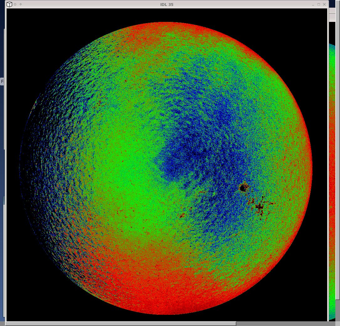
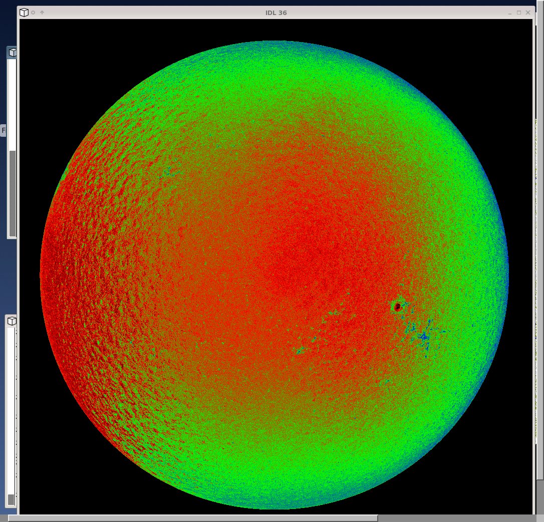
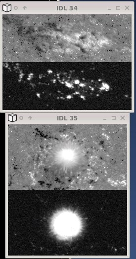
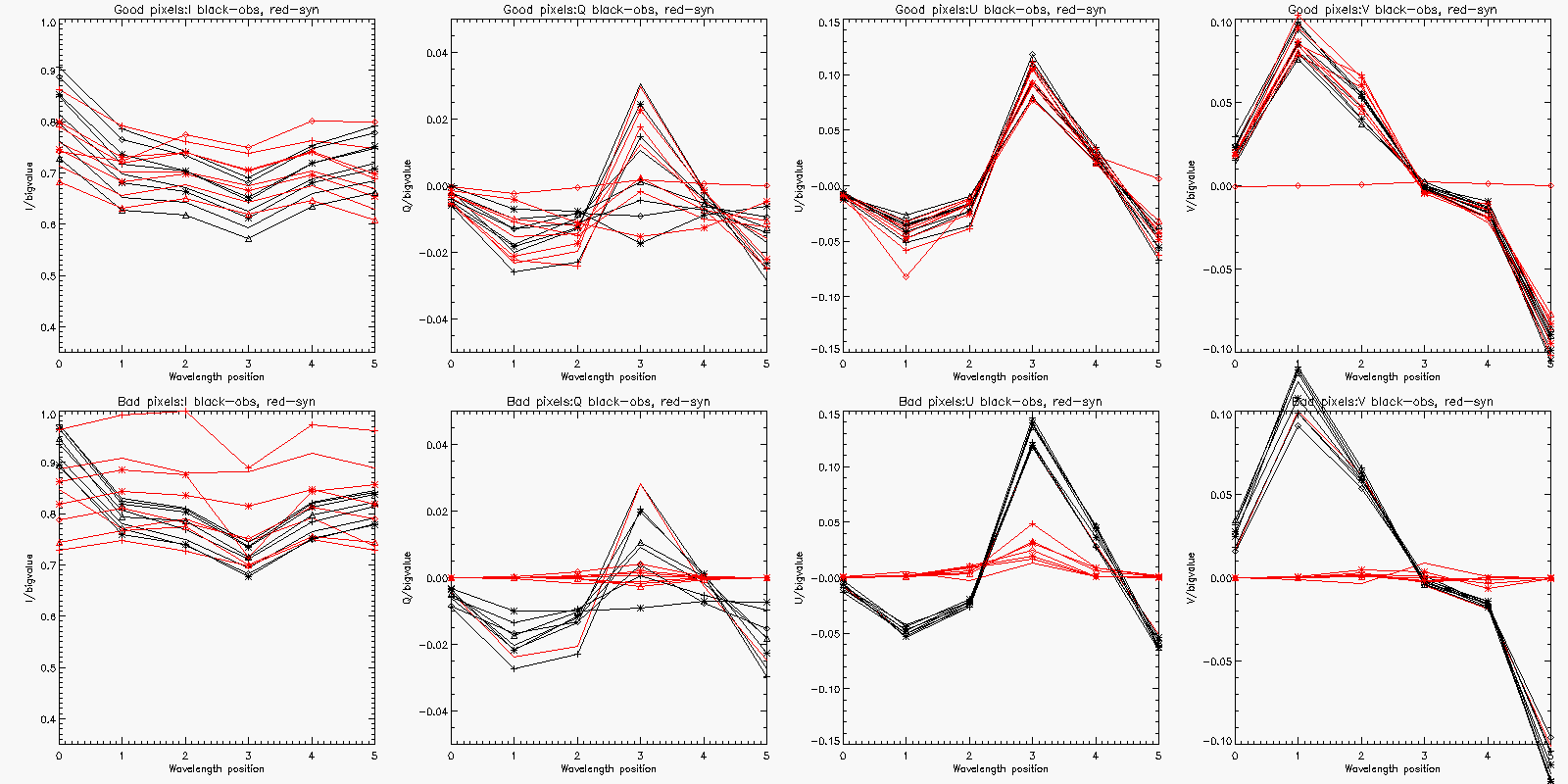
This behavior is actually very similar to what you see with many data sets (e.g., ASP with HAO inversion code, Hinode/SP with MERLIN, etc.). It also appears when with S5 data series (see the figure below: Top pair: May data, bottom: july, both from S5, for each pair, top; inclination angle, bottom: field strength scaled to saturate at 1000.).
Summary: "bad pixels" are seen in umbrae, sometimes also seen in penumbrae and
in quiet Sun (?). Usually inversion fails to fit Stokes QUV. reasons: low intensity--not likely because the
very adjacent pixels return reasonable inversion results. Those pixels have similar values of Stokes IQUV as
that of "bad pixels".
HMI data from Aug. 1 to Oct. 13, and from Dec. 15 to Jan 17 are surveyed. 17 sunspots are examined.
1. Two types of bad pixels: pixels in sunspot umbrae, and pixels outside of the umbrae (in or close to the penumbrae).
2. Bad pixels appear more often outside of sunspot umbrae than in umbrae. 4 of 17 sunspots have bad pixels in umbrae (last up to 4 days, but most within one or two days); more than half have bad pixels outside of the umbrae;
3. For the umbrae's bad pixels, they don't occur during the entire disk passage of the sunspot, but rather only appear when the sunspots approach to the limb.
4. For the umbrae's bad pixels, they could appear individually or in patch;
5. More serious in the time period of Dec.15 to Jan 17 in terms of : (1) more sunspots have bad pixels in umbrae; (2) bad pixels appear as patch; (3) last longer (2 or 3 days). --> due to use of the outdate instrument profiles?
6. Difference between Blos(lcp-rcp) and Blos(vfisv) evidently shows the bad pixels in umbrae but not outside of umbrae.
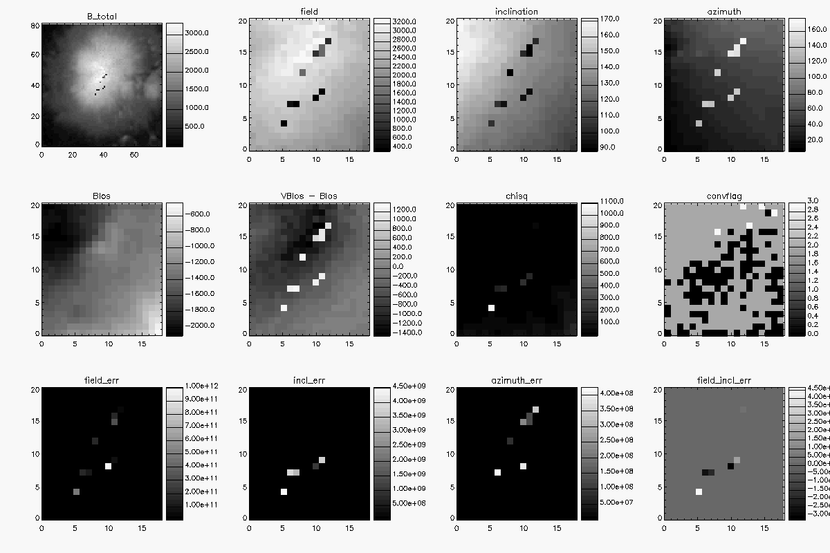
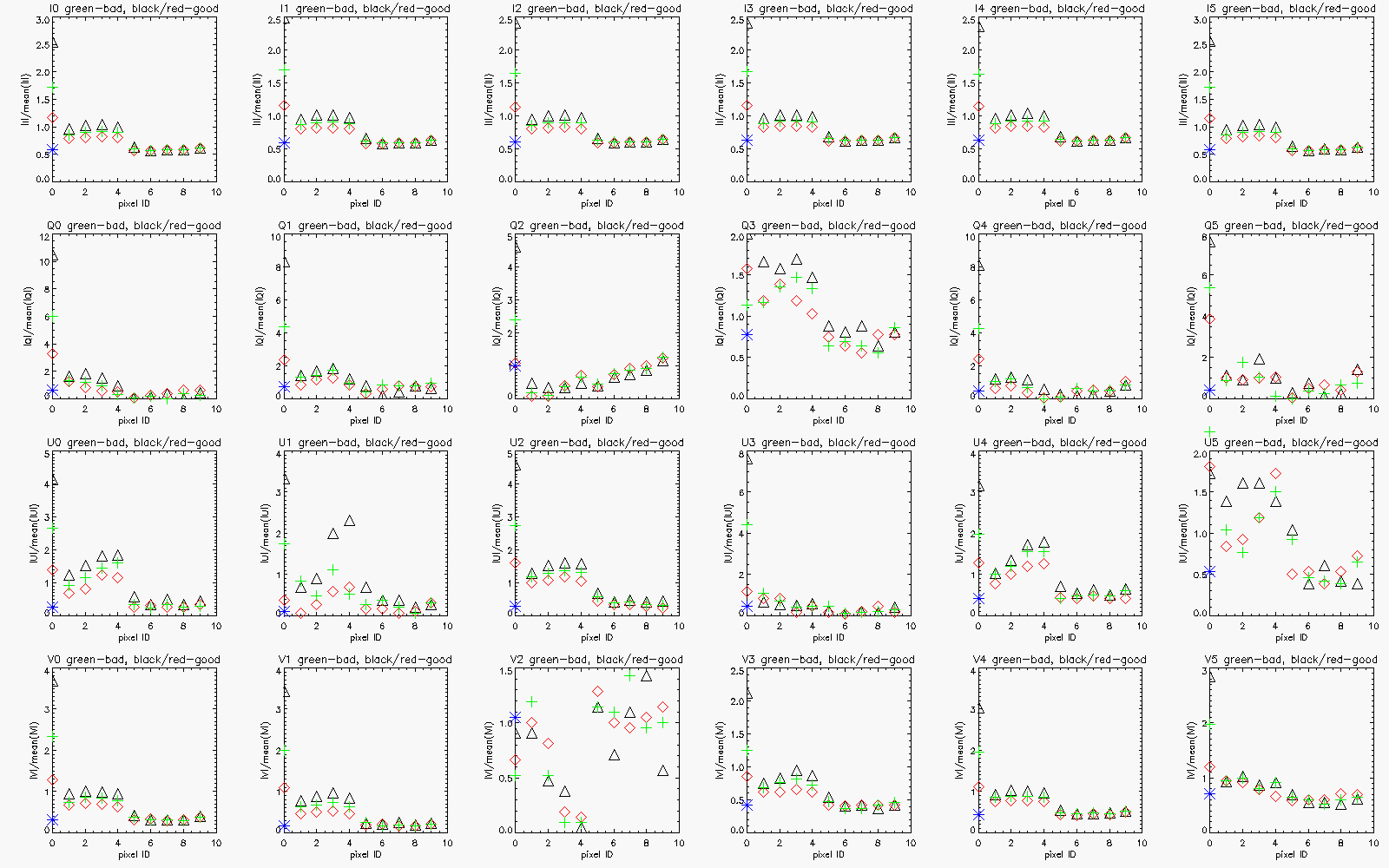
iquv_badpixels_aug01.bmp and iquvbadpixels_jan03.bmp, as you can see, show the inverted field, as well as IQUV at 6 wavelengths for the sunspot on August 1 and Janary 03, respectively. The plot plot_iquvbadpixels_aug01.bmp shows IQUV of the ``bad pixels'' of Aug. 01 data, together with the very adjacent good pixels (upper and lower). All the values are scaled by the median value. The blue stars in these panel refer to the pixel with the maximum field strength in that subimage, as a reference. Mostly, the values of the ``bad pixels'' are just within the values of the two adjacent pixels.
plot_iquvbadpixels_jan03.bmp is in similar format but the good pixels are not necessary very adjacent to the bad pixels because the bad pixels patch together. Again, the values of the ``bad pixels'' are within the range of the good pixels.
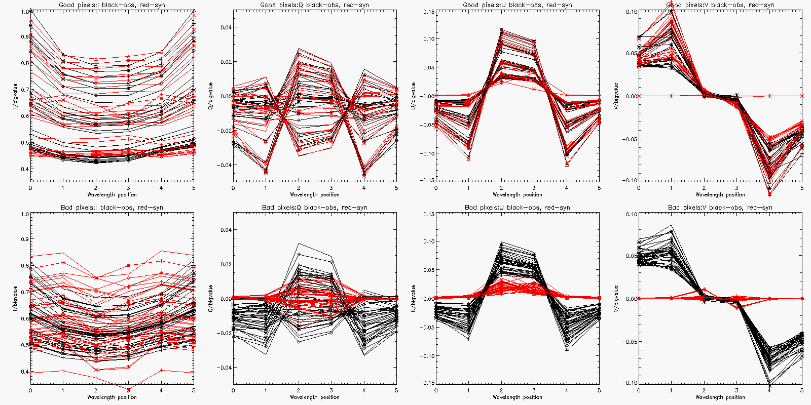
Synthetic line profiles are plotted to compare with the observational data for the good pixels and bad pixels. Basically, the fitting for the bad pixels is very poor. Here is a summary:
1. The number of the ``bad pixels'' doesn't increase with the orbital speed;
2. For ``bad pixels'', the model fails to fit the QUV. But for one case, the synthetic U and V fit observation well, while Q is off (see jan03dusk_1300UT_Stokeprof.bmp);
3. For some ``good pixels'', the synthetic profiles don't fit observation well. The method to identify the ``bad pixels'' seems not very effective. Will look into it.
Another kind of ``bad pixel''. not sure if they have been solved or not. Anyway, here they are.
I've been looking more carefully at the results of the disambiguation for the May interval. In the process, I found discontinuous patches of the output from the inversion in areas other than the umbra of sunspots. Attached are images of the field strength (scaled between 0G and 1000G) and the inclination angle (scaled between 0degree and 90degree) for a small part of AR 11067 on May 04 at 08:00. I think the patches are more clearly seen in the inclination angle, but they also appear to be present in the field strength. Maybe this has already been recognized, but based on the telecon yesterday, it sounded like we were thinking that these patches only occur in the umbra.
 field strength file
 inclination file
Summary: due to background velocity?
Near the limb there seems to be a fairly strong correlation between the medium-scale patterns in field strength and l-o-s velocity. Is that something we can eventually compensate for?
True. I have not looked at it in detail. Is it something that didn't happen before? In that case, I would imagine it's a consequence of the weighting scheme not being optimum in that field strength-intensity regime.
That's probably the lack of a full spectral line sampling, or something like the line center being close to some limit which makes other parameters such as field strength or other thermodynamic parameters need to compensate in order to fit the data.
Summary: this preference is minimized greatly with S4. No
test has been done with S5.
(From Kd.)
We described how obviously different May data looked; there are now plots from the inverted patches on 04 may (xudong_test_patch_vec_4/2010.05.04_00:00:00_TAI_1 and TAI_6) and I think it's pretty clear in the weak-signal areas what we were talking about with regards to preferred directions, and that it is more obvious on this day than in the July data. see May_04_patch1.jpeg and May_04_patch6.jpeg, compare to weak areas in either shown in plage_qs_comp_S3vS4.jpeg.
It's likely due to the different noise levels of Q and U.
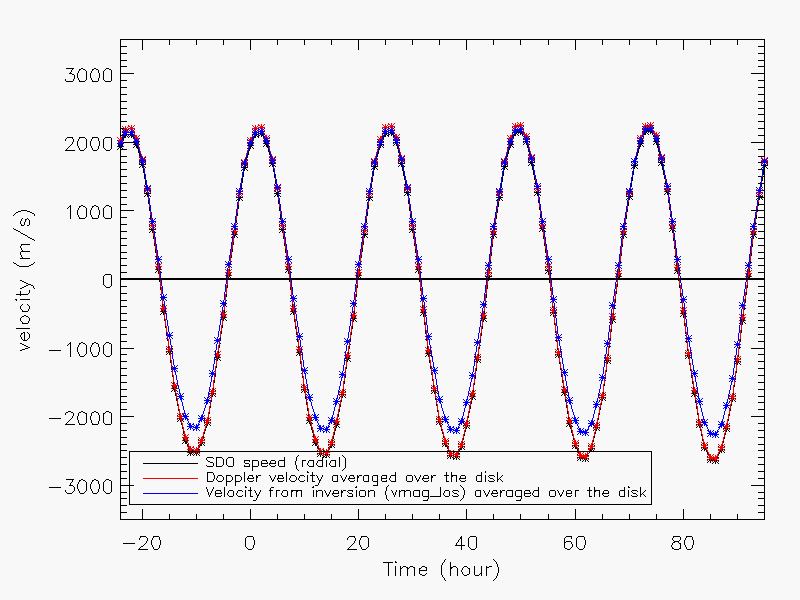
Summary: Vlos_mag (line-of-sight velocity returned from inversion code) appears to
systematically shift towards positive value.
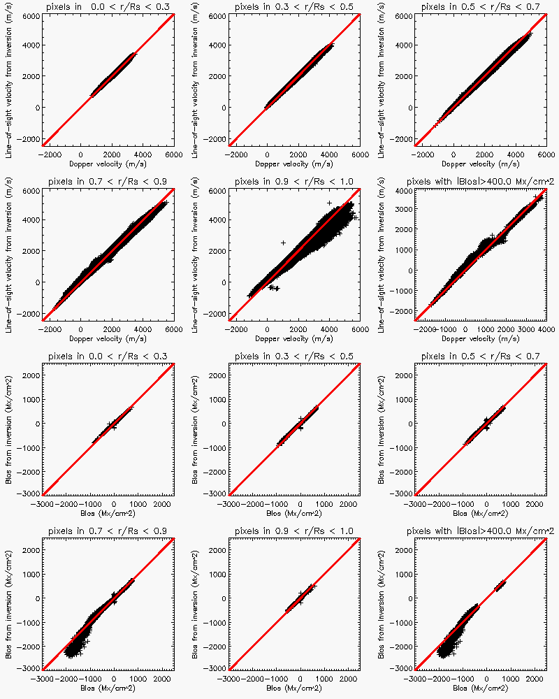
Comparison is done between the average velocities from dopplergrams, inverted line-of-sight velocity (vlos_mag) with the orbital velocity (OBS_VR, defined as ''velocity of the observer in radial direction. + is away from Sun''). The data are from 2010.07.31_00:00:00 to 2010.08.04_23:00:00. The average was done over the pixels within 0.80 Rs.
Scatter plots are presented in Figure between the line-of-sight velocity from Dopplergrams and inverted vlos_mag (top 2 rows) for different areas, and between the line-of-sight magnetic field from LCP/RCP and inverted field (bottom 2 rows). Significant discrepancy can be seen.