Test simulations : MHD/HD with Godunov/Roe-type Riemann solver, TVD, MUSCL etc.

• Orszag-Tang vortex test problem [Orszag and Tang, J. Fluid Mech. (1979)], 2D-MHD, with TVD-MUSCL method

  mpeg, mp4

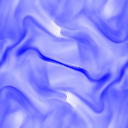
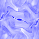
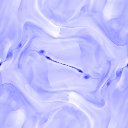
  Snapshot at time ∼ π : The animation movie shows the temperature for the normalized time 0 to 10, simulated with 256x256 grids covering 2π-by-2π space. The colors in the movie runs from 0.2(white) to 1.2(dark blue) in dimensionless value, divided by 0.6 (the initial value of temperature).

  The small-scale discontinuities and vortices, especially at chaotic regime t > 5, are really sensitive to choices of mesh size and computation scheme. The images below show the temperature at t = 7 simulated with, from the left, 64x64, 128x128, 256x256, 512x512 grids, respectively. The identical method, the TVD-MUSCL and the Powell correction of divergence B, was applied. Mind that colors range from the minimum to the maximum in each frame thus do not represent absolute numbers.
  
  
• MHD aligned rotor [c.f. Balsara and Spicer, JCP vol.149 pp.270-292 / vol.153 p.671 (1999)], 2D-MHD, with TVD-MUSCL method.

  Left plot and the background image of this page show the snapshot of temperature at t ∼ 1 and 1.5, respectively.

  
  
• Interaction between oblique MHD shock and dense cloud [c.f. Dai and Woodward, ApJ vol.494 p.317 (1998)], 2D-MHD, with TVD-MUSCL method

  Temperature at t ~ 0.055.

  
  
• Kelvin-Helmholtz Instability, 2D-MHD, with TVD-MUSCL method
  The hydrodynamics case is very chaotic, as seen in this movie (mpeg or mp4). The below are snapshots of temperature at t = 0, 1/2, 1, 2, 5. Here a small mass density enhancement, instead of small random flow, is given at the lower border to induce/seed instability. Under the presence of the magnetic field, results are quite different. Plots, show the simulated temperature at t = 0, 1 and 4 (with 256x256 grids) of the weakly-magnetized plasma. A uniform horizontal field (beta-ratio is 20) is given as the initial field. The initial plasma (t = 0) is identical to the HD case above. This movie (mpeg or mp4) shows temperature at t = 0 ∼ 10. Magnetic field works to stabilize system, suppressing the evolution of small-scale instabilities.
  
  
• Rayleigh-Taylor instability, 2D-HD/MHD, with TVD MUSCL method

  HD case mpeg, mp4

  Vertical mpeg, mp4

  Horizontal mpeg, mp4

  Oblique mpeg, mp4

  From left shown are the snapshots at t ∼ 12.75 of hydrodynamics case (without magnetic field), and three magnetohydrodynamics cases starting with vertical, horizontal and oblique magnetic field. The initial magnetic field in all MHD cases is uniform and, its strength is set so that the beta ratio will be 250 at the boundary between the high- and low-density regimes. All four cases start with the identical initial plasma distribution with tiny "single"-mode symmetric fluctuation of bulk flow. The movies in the left show the temporal evolutions from t = 0 to 15. Here again, (tension of) magnetic field works to suppress instability with different ways depending on the direction of field.

  
  

  mpeg, mp4

  When the initial magnetic field has only the component perpendicular to the plotted plane, the magnetic field will behave as if it is a plasma with specific heat ratio of 2. In this case, no magnetic tension will arise, and thus instability will not be suppressed.

  
  

  HD case mpg, mp4

  MHD case mpeg, mp4

  The evolutions of RT instability of HD (left) and MHD (right) cases starting with multiple-wavelength small-amplitude fluctuations of plasma : The MHD case starts with uniform, horizontal, and very weak magnetic field (beta-ratio is about 1000).

  
  
• 1-D MHD shock/discontinuity problem with TVD-MUSCL method [c.f. Ryu and Jones, ApJ vol.442 p.228-258 (1995)],

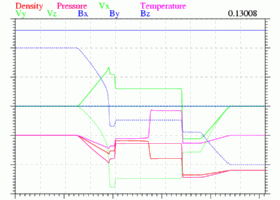  mpeg, mp4

  The initial values at left and right side, in a order [Rho, Vx, Vy, Vz, Bx, By, Bz, Pg], are [1, 0, 0, 0, 1.3, 1.0, 0, 1.0] and [0.4, 0, 0, 0, 1.3, -1, 0, 0.4], respectively. The specific heat ratio (γ) is set to be 5/3. The non-reflection boundary treatment based on the method of characteristics is applied at both ends.

• 2-D MHD, lens for MHD waves with TVD-MUSCL method

  mpeg, mp4

  A plane pressure perturbation is given to the left side of plano-convex/concave magnetic lens with the magnetic field vector perpendicular to the plane. Being set the background plasma temperature and total pressure constant (except the pressure-perturbation site), the wave driven by the pressure perturbation propagates rightward then undergoes refractions at the contact with the magnetic column. Because the propagation speeds inside the lens are faster than the one outside, the refractions are in opposite sense than the optic ones. The left plot and movies show the temporal evolution of the gas pressure (propagating from left to right).

Other test simulations

• Non-reflection boundary treatment by means of the projected normal characteristics method [c.f. Nakagawa, (1980); Wu et al., (1983); Han et al., (1988)]

  mpeg, mp4

  mpeg, mp4

  The two plots show the snapshot of the gas pressure; the MHD (left) and HD(right) waves propagate, responding to the impulse given at the center. The non-reflection boundary treatment based on the "projected normal characteristics method" is implemented on the four "free" boundaries which limit the domain of computation. Mainly because this method uses only the normal component of the characteristic curves for simplicity, reflection slightly remains. However, most of wave energy goes outside the computation domain, and such small reflection waves vanish after reflecting twice or so.

  The projected normal characteristics method can provide MHD/HD solution at the outermost grids satisfying the governing (hyperbolic) equations and the concept of the characteristics. In analogy, this boundary treatment provides the simulations with "anechoic chamber" environment, and at the same time, its ability of discarding non-physical waves coming from outside provides quietness like the one "noise-cancellation" headphone provides.
  With some modification and adjustment, this method and concept can be straightforwardly applied to the "physical boundary" where physically meaningful values, conditions and constraints are specified. Specifically this is very helpful for the simulation studies of the solar corona in which we often use the observational values as the boundary values on the sub-Alfvenic solar surface (or photosphere or "coronal base" at some height).
  
  
• WENO (weighted essentially non oscillatory) method (5th-order) [c.f. Jiang and Wu, JCP vol. 150-2 pp.561-594(1999)]

  The snapshots of Orszag-Tang vortex problem at time ∼ π.    The left plot is a snapshot of the simulated temperature with the 5th-order weighted essentially non-oscillatory (WENO) method and the Roe's method. The right one is obtained with 3rd-order TVD-MUSCL (here, with "minmod" function) and thus identical to the plot appearing in the topmost part of this page.

     Both schemes work pretty well for solving many kinds of MHD/HD problems, and there seem few differences between the two cases. Looking at details, though, we can find some. With the Roe-type method, the nonlinear steepening at shock discontinuity is better treated. The WENO and its earlier version, ENO, can better preserve the maximum and minimum values of spatially smoothed curves (like sinusoidal). The WENO-Roe is a combined version of these two methods, picking up virtues of each.
  
  
• HLL (Harten-Lax-van Leer) approximate Riemann solver.
  ... and
  HLLC (HLL contact ; [Toro,E.F., Spruce,M. and Speares,W.]),
  HLLD (HLL discontinuities ; [Miyoshi,T and Kusano,K., J.Comp.Phys. vol.136 p.315 (2005)],)
  coming soon ...
• CT (constraint transport) method
  ... for always satisfying the divergence-free constraint of the magnetic field governed by induction equation.
  coming soon ...
• Conjugate Gradient method(s)
  This method (or a group of methods) of the matrix inversion algorithm is widely used in the fast-and-efficient Laplace or Poisson solvers. This may have advantages for improving performance of the MHD/HD simulations.
  coming soon ...

Other simulations : … just for fun

• Particle motions in the two-dimensional hydrodynamical flow.

  mpeg, mp4

  An asymmetric heat source is given on the bottom boundary to induce asymmetric motions. Particle motions are traced with Runge-Kutta method.    The Lax-Wendroff method is numerically diffusive, though, has been long used because it is simple and much less computationally expensive. Computations with this method are generally 4 ∼ 6 times faster than those with the TVD method of Godunov type approximate Riemann solver. This is an advantage for various simulation problems.

  
  
• Supersonic flow (M=10) injection, 2D-HD, with Rusanov/Lax-Friedrichs method

  mpeg, mp4

  A tiny density enhancement is given near the injection site (on the left boundary), so that symmetry will be broken. With a very-simplified Riemann solver, the Lax-Friedrichs method is a quick but sufficiently accurate scheme.

  
  
• Collision of two fluid bodies, 2D-HD, Godunov TVD-MUSCL

  mpeg, mp4

  Just for fun.    Collision of two objects is simulated with compressive fluid code. With the initial pressure being uniform everywhere in the simulation box, the objects are featured by different density (thus, different temperature) values. The ratio of initial densities at the core (inner part) of the left object, the outer part of the left object, the right object, and the surrounding space, is 20 : 10 : 15 : 1. The right object is moving leftward to collide onto the left one. Periodic boundary is applied on all four boundaries. No gravity is taken into account.