There are two simple and straightforward ways to render three-dimensional scalar data. One is to draw the contour surface. In order that images will look natural to our eyes, a light source will be set, and the reflection and scattering on the surface be considered to calculate color and brightness. The other way is line-of-sight integration of values to make "ghost" or "fog", which allows us to see objects behind objects. Optical depth may be taken into account if necessary. In many cases, it is convenient to use the normalized values of the scalar data ranging from 1 to 0. I used "arc-tangent" to define a "good" step-wise function to rescale the values; it is written as
where the value varies quickly and smoothly from 0 to 1
around a0 with adequately small positive ε.
Thus, the stepwise above determines whether
a point (x,y,z) is inside (= 1) or outside (= 0) of
contour surface a(x,y,z) = a0.
Any other step-wise functions may work for rescaling/normalizing,
though, arc-tangent may be best because it is continuous,
symmetric, and calculable for any input (of real number).
In addition, with the step-wise function above, we can do some kind of logical operation;
adding the functions is equivalent to logical operation "OR",
multiplying is to "AND",
and minus sign (or an operation a'=1-a) works as "NOT".
Dividing is of no meanings here.
 ,
of an image,
,
of an image,
 (mp4)
is expressed as
(mp4)
is expressed as
 .
.
The first line defines an infinite column with radius of 0.18 centered along x-axis.
The second gives lower limit to the range of x (x > -0.88), and
the third does upper limit (x < +0.88).
With these three lines multiplied, one finite column is defined.
Line 4 defines a sphere with radius of 0.22 near one end of the column (centered at (1,0.15,0)),
and this sphere will be "added" in the plot because line 4 is added in the equation of the scalar function.
Three other balls are added to complete the white part drawn above, and
the brawn part is defined in a way similar.
It is a fun; logical operation here is like clay-playing,
and you can make animation by accordingly combining the still images.
I like this.
To make a sort of three-dimensional view, the z-buffer strategy is applied here.
We first define a projection plane and lattice (pixel) dimensions.
First, we define a line of sight, which must pass a viewing point and center of a lattice on the projection plane.
Then, calculating the scalar values along the line of sight, from the viewing point, we can find a point at which the scalar value crosses a certain threshold value.
In a definition above (with a lot of arctans), the threshold must be a float number between 0.0 and 1.0.
By doing the same thing along another line starting from the intersection to a light source,
you can know whether or not the intersection point is in a shadow of the other part of object.
If necessary, you may calculate the normal vector of the contour surface (minus gradient of scalar), inner (dot) product with the line-of-sight vector, and other attributes at the intersecting point
with which we can at last calculate a set of color and brightness values at a pixel.
Effects in optics such as reflection and scattering many be taken into account for better visual effects.
All below in this page and many of visualizations shown in my other pages
(under http://sun.stanford.edu/~keiji/)
were made in this way (a bit more specifically, with FORTRAN 77 or 90,
without any third-party libraries).
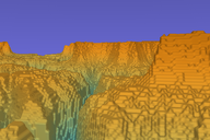 grand canyon (i) mp4 flying in good visibility |
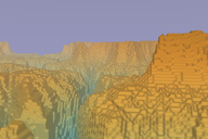 grand canyon (ii) mp4 flying in fog |
 duck mp4 peace |
 hare mp4 animal of 2023 |
 cake mp4 happy birthday |
 pumpkin mp4 happy Halloween |
 cheese (i) mp4 cheese rotating. mice might like this |
 cheese (ii) mp4 cheese evaporating |
 cheese (iii) mp4 cheese, from fly's point of view |
 vessel mp4 |
 spiral shell mp4 |
 plane and sphere mp4 |
 box mp4 |
 worm mp4 bird may like this |
 optically thin mp4 |
 optically thick mp4 |
 game of life mp4 in reality, more complicated |
 fireworks mp4 happy holiday! |